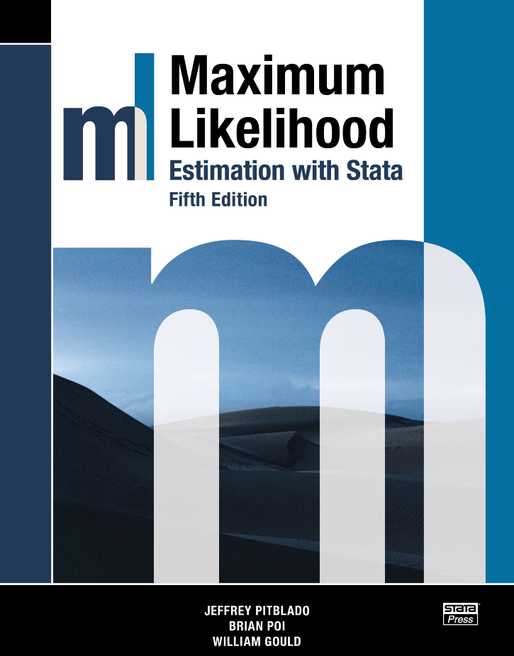
Maximum Likelihood Estimation with Stata, Fifth Edition
121,000원
Authors: Jeffrey Pitblado, Brian Poi, and William Gould
Publisher: Stata Press
Copyright: 2024
ISBN-13: 978-1-59718-411-3
Pages: 472; paperback
Preface to the Fifth Edition
Author index
Subject index
Download the datasets used in this book
Maximum Likelihood Estimation with Stata, Fifth Edition is the essential reference and guide for researchers in all disciplines who wish to write maximum likelihood (ML) estimators in Stata. Beyond providing comprehensive coverage of Stata's command for writing ML estimators, the book presents an overview of the underpinnings of maximum likelihood and how to think about ML estimation.
The fifth edition includes a new second chapter that demonstrates the easy-to-use mlexp command. This command allows you to directly specify a likelihood function and perform estimation without any programming.
The core of the book focuses on Stata's ml command. It shows you how to take full advantage of ml’s noteworthy features:
- Linear constraints
- Four optimization algorithms (Newton–Raphson, DFP, BFGS, and BHHH)
- Observed information matrix (OIM) variance estimator
- Outer product of gradients (OPG) variance estimator
- Huber/White/sandwich robust variance estimator
- Cluster–robust variance estimator
- Complete and automatic support for survey data analysis
- Direct support of evaluator functions written in Mata
When appropriate options are used, many of these features are provided automatically by ml and require no special programming or intervention by the researcher writing the estimator.
In later chapters, you will learn how to take advantage of Mata, Stata's matrix programming language. For ease of programming and potential speed improvements, you can write your likelihood-evaluator program in Mata and continue to use ml to control the maximization process. A new chapter in the fifth edition shows how you can use the moptimize() suite of Mata functions if you want to implement your maximum likelihood estimator entirely within Mata.
In the final chapter, the authors illustrate the major steps required to get from log-likelihood function to fully operational estimation command. This is done using several different models: logit and probit, linear regression, Weibull regression, the Cox proportional hazards model, random-effects regression, and seemingly unrelated regression. This edition adds a new example of a bivariate Poisson model, a model that is not available otherwise in Stata.
The authors provide extensive advice for developing your own estimation commands. With a little care and the help of this book, users will be able to write their own estimation commands—commands that look and behave just like the official estimation commands in Stata.
Whether you want to fit a special ML estimator for your own research or wish to write a general-purpose ML estimator for others to use, you need this book.
Jeff Pitblado is Executive Director, Statistical Software at StataCorp. Pitblado has played a leading role in the development of ml: he added the ability of ml to work with survey data, and he wrote the current implementation of ml in Mata.
Brian Poi previously worked as a developer at StataCorp and wrote many popular econometric estimators in Stata. Since then, he has applied his knowledge of econometrics and statistical programming in several areas, including macroeconomic forecasting, credit analytics, and bank stress testing.
William Gould is President Emeritus of StataCorp and headed the development of Stata for over 30 years. Gould is also the architect of Mata.
List of tables
1.2 Likelihood theory
1.2.2 Likelihood-ratio tests and Wald tests
1.2.3 The outer product of gradients variance estimator
1.2.4 Robust variance estimates
The Newton–Raphson algorithm
The DFP and BFGS algorithms
1.3.4 Numerical derivatives
1.3.5 Numerical second derivatives
2.2 Normal linear regression
2.3 Initial values
2.4 Restricted parameters
2.5 Robust standard errors
2.6 The probit model
2.7 Specifying derivatives
2.8 Additional estimation features
2.9 Wrapping up
3.2 Normal linear regression
3.3 Robust standard errors
3.4 Weighted estimation
3.5 Other features of method-gf0 evaluators
3.6 Limitations
4.2 Equations in ml
4.3 Likelihood-evaluator methods
4.4 Tools for the ml programmer
4.5 Common ml options
4.5.2 Weights
4.5.3 OPG estimates of variance
4.5.4 Robust estimates of variance
4.5.5 Survey data
4.5.6 Constraints
4.5.7 Choosing among the optimization algorithms
4.7 Appendix: More about scalar parameters
5.2 Examples
5.2.2 Normal linear regression
5.2.3 The Weibull model
5.4 Problems you can safely ignore
5.5 Nonlinear specifications
5.6 The advantages of lf in terms of execution speed
6.2 Outline of evaluators of methods lf0, lf1, and lf2
6.2.2 The b argument
6.2.4 Arguments for scores
6.2.5 The H argument
6.3.2 Method lf1
6.3.3 Method lf2
6.4.2 Normal linear regression
6.4.3 The Weibull model
7.2 Outline of method d0, d1, and d2 evaluators
7.2.2 The b argument
7.2.3 The lnf argument
Using mlsum to define lnf
7.3.2 Method d1
7.3.3 Method d2
7.4.2 Calculating g
7.4.3 Calculating H
8.2 Using the debug methods
8.2.2 Second derivatives
9.2 ml plot
9.3 ml init
10.2 Pressing the Break key
10.3 Maximizing difficult likelihood functions
11.2 Redisplaying output
12.2 Puttinig the do-file into production
13.2 The standard estimation-command outline
13.3 Outline for estimation commands using ml
13.4 Using ml in noninteractive mode
13.5.2 Estimation subsample
13.5.3 Parsing with help from mlopts
13.5.4 Weights
13.5.5 Constant-only model
13.5.6 Initial values
13.5.7 Saving results in e()
13.5.8 Displaying ancillary parameters
13.5.9 Exponentiated coefficients
13.5.10 Offsetting linear equations
13.5.11 Program properties
14.2 Writing your own predict command
15.1.2 The Weibull model
lf-family evaluators
d-family evaluators
Obtaining model parameters
Summing individual or group-level log likelihoods
Calculating the gradient vector
Calculating the Hessian
15.4.2 Calculating g
15.4.3 Calculating H
15.4.4 Results at last
16.1.2 The Weibull model
16.2.2 Not using moptimize_init_touse()
16.3.2 Panel data and clusters
16.3.3 Survey data
16.3.4 Initial values
16.5 Results
16.5.2 Retrieving results
16.5.3 Storing results in e()
16.6.2 Initial values
16.6.3 Constraints
17.2 The probit model
17.3 Normal linear regression
17.4 The Weibull model
17.5 The Cox proportional hazards model
17.6 The random-effects regression model
17.7 The seemingly unrelated regression model
17.8 A bivariate Poission regression model
17.8.2 Bivariate Poisson regression
17.8.3 Discussion
D.2 Method d0
D.3 Method d1
D.4 Method d2
D.5 Method lf0
D.6 Method lf1
D.7 Method lf2
E.2 The probit model
E.3 The normal model
E.4 The Weibull model
E.5 The Cox proportional hazards model
E.6 The random-effects regression model
E.7 The seemingly unrelated regression model
E.8 A bivariate Poisson regression model


