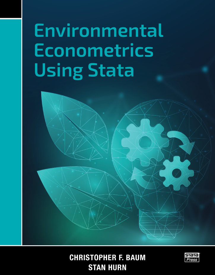
Environmental Econometrics Using Stata
121,000원
Authors: Christopher F. Baum and Stan Hurn Publisher: Stata Press Copyright: 2021 ISBN-13: 978-1-59718-355-0 Pages: 416; paperback
Environmental Econometrics Using Stata is written for applied researchers that want to understand the basic theory of modern statistical methods and how to use them. It is also perfectly suited for teaching. Each chapter is motivated with real data and ends with a set of exercises. The book is also inherently interdisciplinary. The questions posed by environmental issues are relevant to researchers in the physical sciences, economics, sociology, political science, and public health, among other fields.
Each chapter begins with a real dataset and research question. The authors then provide a gentle introduction to the statistical method and demonstrate how to use it to answer the research question. The authors discuss the assumptions about the data and the model, demonstrate the Stata commands used to fit the model and check the model assumptions, and interpret the results. The workflow of the book mimics the workflow that would be required to present your results to an academic audience.
The book is of interest not only for its exposition of the topics but also for its breadth. The book presents estimators for continuous, binary, and ordered outcomes in cross-sectional data; univariate and multivariate time series with stationary and nonstationary data; linear and dynamic panel data; and spatial models and fractional integration. The range of methods is not arbitrary; it is a function of the questions posed by environmental data and reflects the challenges faced by researchers from different disciplines to answer a wide range of questions using modern statistical methods.
Christopher F. Baum is a professor of economics and social work at Boston College. Baum has taught econometrics for many years, using Stata extensively in academic and nonacademic settings. He has over 40 years of experience with computer programming and has authored or coauthored several widely used Stata commands. He is the author of An Introduction to Modern Econometrics Using Stata and An Introduction to Stata Programming, Second Edition. He is an associate editor of the Stata Journal and maintains the Statistical Software Components Archive of community-contributed Stata materials.
Stan Hurn is a professor of econometrics at Queensland University of Technology. He held previous positions at the University of Glasgow and at Brasenose College, Oxford. He is a fellow of the Society for Financial Econometrics. His main research interests are in the field of time-series econometrics, and he has been published widely in leading international journals. He is also the coauthor of Econometric Modelling with Time Series: Specification, Estimation and Testing and Financial Econometric Modeling.
1.1.2 Nonlinearity
1.1.3 Structural breaks and nonstationarity
1.1.4 Time-carrying volatility
Types of data
2.2 Linear regression and OLS estimation
2.3 Interpreting and assessing the regression model
Tests of significance
2.3.2 Residual diagnostics
Homoskedasticity
Serial independence
Normality
3.2 Properties of estimators
Asymptotic normality
Asymptotic efficiency
3.4 Hypothesis testing
Wald test
LM test
3.6 Testing for exogeneity
4.2 Specifying and fitting dynamic time-series models
Moving-average models
ARMA models
4.4 ARMA models for load-weighted electricity price
4.5 Seasonal ARMA models
5.2 The VARMA model
5.3 The VAR model
5.4 Analyzing the dynamics of a VAR
5.4.2 Impulse–responses
Vector moving-average form
Orthogonalized impulses
5.4.3 Forecast-error variance decomposition
5.5.2 Long-run restrictions
6.2 Unit roots
6.3 First-generation unit-root tests
6.3.2 Phillips–Perron tests
6.4.2 Elliott–Rothenberg–Stock DFGLS test
6.5.2 Single-break unit-root tests
6.5.3 Double-break unit-roots tests
7.2 Illustrating equilibrium relationships
7.3 The VECM
7.4 Fitting VECMs
7.4.2 System estimation
7.6 Cointegration and structural breaks
8.2 Introductory terminology
8.3 Recursive forecasting in time-series models
8.3.2 Multiple-equation forecasts
8.3.3 Properties of recursive forecasts
8.5 Daily forecasts of wind speed for Santiago
8.6 Forecasting with logarithmic dependent variables
8.6.2 Generalized linear models
9.2 The Kalman filter
9.3 Vector autoregressive moving-average models in state-space form
9.4 Unobserved component time-series models
9.4.2 Seasonals
9.4.3 Cycles
10.2 Testing
10.3 Bilinear time-series models
10.4 Threshold autoregressive models
10.5 Smooth transition models
10.6 Markov switching models
11.2 The generalized autoregressive conditional heteroskedasticity model
11.3 Alternative distributional assumptions
11.4 Asymmetries
11.5 Motivating multivariate volatility models
11.6 Multivariate volatility models
11.6.2 The dynamic conditional correlation model
12.2 Data organization
12.2.2 Reshaping the data
12.4 Fixed effects and random effects
12.4.2 Two-way FE
12.4.3 REs
12.4.4 The Hausman test in a panel context
12.4.5 Correlated RE
13.2 The spatial weighting matrix
Distance weights
Contiguity weights
13.2.2 Construction
13.4 Spatial models
Spatial error model
Spatial error model
13.7 Model selection
14.2 The data
14.3 Binary dependent variables
14.3.2 Binomial logit and probit models
14.5 Censored dependent variables
15.2 Autocorrelations and long memory
15.3 Testing for long memory
15.4 Estimating d in the frequency domain
15.5 Maximum likelihood estimation of the ARFIMA model
15.6 Fractional cointegration
A.1.2 Organization of do-, ado-, and data files
A.1.3 Editing Stata do- and ado-files
A.2.2 Getting your data into Stata
Handling text files
The import delimited command
Accessing data stored in spreadsheets
Importing data from other package formats
A.2.3 Other data issues
Protecting the data in memory
Missing data handling
Recoding missing values: the mvdecode and mvencode commands
A.2.4 String-to-numeric conversion and vice versa
Observation numbering: _n and _N
The varlist
The numlist
The if exp and in range qualifiers
Local macros
Global macros
Scalars
Matrices
Looping
The generate command
The egen command
Computation for by-groups
Time-series operators
A.6 Circular variables

