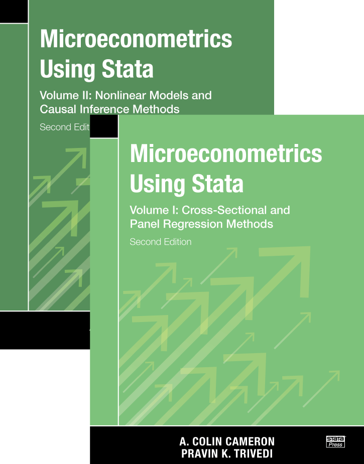
Microeconometrics Using Stata, Second Edition
293,000원
Volume I: Cross-Sectional and Panel Regression Methods
Volume II: Nonlinear Models and Causal Inference Methods
Authors: A. Colin Cameron and Pravin K. Trivedi Publisher: Stata Press Copyright: 2022 ISBN-13: 978-1-59718-359-8 Pages: 1,675; paperback Volume I: Cross-Sectional and Panel Regression Methods
ISBN-13: 978-1-59718-361-1 Pages: 817; paperback
Volume II: Nonlinear Models and Causal Inference Methods
ISBN-13: 978-1-59718-362-8 Pages: 858; paperback
Every applied economic researcher using Stata and everyone teaching or studying microeconometrics will benefit from Cameron and Trivedi's two volumes. They are an invaluable reference of the theory and intuition behind microeconometric methods using Stata. Those familiar with Cameron and Trivedi's Microeconometrics: Methods and Applications will find the same rigor. Those familiar with the previous edition of "Microeconometrics Using Stata" will find the familiar focus on Stata commands, their interpretation, and their connection with microeconometric theory as well as an introduction to computational concepts that should be part of any researcher's toolbox. And readers will find much more—so much more, the second edition required a second volume.
This new edition covers all the new Stata developments relevant to microeconometrics that appeared since the the last edition in 2010. For example, readers will find entire new chapters on treatment effects, duration models, spatial autoregressive models, lasso, and Bayesian analysis. But the authors didn't stop there. They also added discussions of the most recent microeconometric methods that have been contributed by the Stata community.
The first volume introduces foundational microeconometric methods, including linear and nonlinear methods for cross-sectional data and linear panel data with and without endogeneity as well as overviews of hypothesis and model-specification tests. Beyond this, it teaches bootstrap and simulation methods, quantile regression, finite mixture models, and nonparametric regression. It also includes an introduction to basic Stata concepts and programming and to Mata for matrix programming and basic optimization.
The second volume builds on methods introduced in the first volume and walks readers through a wide range of more advanced methods useful in economic research. It starts with an introduction to nonlinear optimization methods and then delves into binary outcome methods with and without endogeneity; tobit and selection model estimates with and without endogeneity; choice model estimation; count data with and without endogeneity for conditional means and count data for conditional quantiles; survival data; nonlinear panel-data methods with and without endogeneity; exogenous and endogenous treatment effects; spatial data modeling; semiparametric regression; lasso for prediction and inference; and Bayesian econometrics.
With its encyclopedic coverage of modern econometric methods paired with many worked examples that demonstrate how to implement these methods in Stata, "Microeconometrics Using Stata, Second Edition" is a text that readers will come back to over and over for each new project or analysis they face. It is an essential reference for applied researchers and those taking microeconometrics courses.
Colin Cameron is a professor of economics at the University of California–Davis, where he teaches econometrics at undergraduate and graduate levels, as well as an undergraduate course in health economics. He has given short courses in Europe, Australia, Asia, and South America. His research interests are in microeconometrics, especially in robust inference for regression with clustered errors. He is currently an associate editor of the Stata Journal.
Pravin K. Trivedi is a Distinguished Professor Emeritus at Indiana University–Bloomington and an honorary professor in the School of Economics at the University of Queensland. During his academic career, he has taught undergraduate- and graduate-level econometrics in the United States, England, Europe, and Australia. His research interests include microeconometrics and health economics. He has served as coeditor of the Econometrics Journal from 2000–2007 and associate editor of the Journal of Applied Econometrics from 1986–2015. He has coauthored (with David Zimmer) Copula Modeling in Econometrics: An Introduction for Practitioners (2007).
Cameron and Trivedi’s joint work includes research articles on econometric models and tests for count data, the Econometric Society monograph Regression Analysis of Count Data, and the graduate-level text Microeconometrics: Methods and Applications.
1.2 Documentation
1.3 Command syntax and operators
1.4 Do-files and log files
1.5 Scalars and matrices
1.6 Using results from Stata commands
1.7 Global and local macros
1.8 Looping commands
1.9 Mata and Python in Stata
1.10 Some useful commands
1.11 Template do-file
1.12 Community-contributed commands
1.13 Additional resources
1.14 Exercises
2.2 Types of data
2.3 Inputting data
2.4 Data management
2.5 Manipulating datasets
2.6 Graphical display of data
2.7 Additional resources
2.8 Exercises
3.2 Data and data summary
3.3 Transformation of data before regression
3.4 Linear regression
3.5 Basic regression analysis
3.6 Specification analysis
3.7 Specification tests
3.8 Sampling weights
3.9 OLS using Mata
3.10 Additional resources
3.11 Exercises
4.2 In-sample prediction
4.3 Out-of-sample prediction
4.4 Predictive margins
4.5 Marginal effects
4.6 Regression decomposition analysis
4.7 Shapley decomposition of relative regressor importance
4.8 Differences-in-differences estimators
4.9 Additional resources
4.10 Exercises
5.2 Pseudorandom-number generators
5.3 Distribution of the sample mean
5.4 Pseudorandom-number generators: Further details
5.5 Computing integrals
5.6 Simulation for regression: Introduction
5.7 Additional resources
5.8 Exercises
6.2 Generalized least-squares and FGLS regression
6.3 Modeling heteroskedastic data
6.4 OLS for clustered data
6.5 FGLS estimators for clustered data
6.6 Fixed-effects estimator for clustered data
6.7 Linear mixed models for clustered data
6.8 Systems of linear regressions
6.9 Survey data: Weighting, clustering, and stratification
6.10 Additional resources
6.11 Exercises
7.2 Simultaneous equations model
7.3 Instrumental-variables estimation
7.4 Instrumental-variables example
7.5 Weak instruments
7.6 Diagnostics and tests for weak instruments
7.7 Inference with weak instruments
7.8 Finite sample inference with weak instruments
7.9 Other estimators
7.10 Three-stage least-squares systems estimation
7.11 Additional resources
7.12 Exercises
8.2 Panel-data methods overview
8.3 Summary of panel data
8.4 Pooled or population-averaged estimators
8.5 Fixed-effects or within estimator
8.6 Between estimator
8.7 Random-effects estimator
8.8 Comparison of estimators
8.9 First-difference estimator
8.10 Panel-data management
8.11 Additional resources
8.12 Exercises
9.2 Panel IV estimation
9.3 Hausman–Taylor estimator
9.4 Arellano–Bond estimator
9.5 Long panels
9.6 Additional resources
9.7 Exercises
10.2 Binary outcome models
10.3 Probit model
10.4 MEs and coefficient interpretation
10.5 Logit model
10.6 Nonlinear least squares
10.7 Other nonlinear estimators
10.8 Additional resources
10.9 Exercises
11.2 Critical values and p-values
11.3 Wald tests and confidence intervals
11.4 Likelihood-ratio tests
11.5 Lagrange multiplier test (or score test)
11.6 Multiple testing
11.7 Test size and power
11.8 The power onemean command for multiple regression
11.9 Specification tests
11.10 Permutation tests and randomization tests
11.11 Additional resources
11.12 Exercises
12.2 Bootstrap methods
12.3 Bootstrap pairs using the vce(bootstrap) option
12.4 Bootstrap pairs using the bootstrap command
12.5 Percentile-t bootstraps with asymptotic refinement
12.6 Wild bootstrap with asymptotic refinement
12.7 Bootstrap pairs using bsample and simulate
12.8 Alternative resampling schemes
12.9 The jackknife
12.10 Additional resources
12.11 Exercises
13.2 Nonlinear example: Doctor visits
13.3 Nonlinear regression methods
13.4 Different estimates of the VCE
13.5 Prediction
13.6 Predictive margins
13.7 Marginal effects
13.8 Model diagnostics
13.9 Clustered data
13.10 Additional resources
13.11 Exercises
14.2 Models based on finite mixtures
14.3 FMM example: Earnings of doctors
14.4 Global polynomials
14.5 Regression splines
14.6 Nonparametric regression
14.7 Partially parametric regression
14.8 Additional resources
14.9 Exercises
15.2 Conditional quantile regression
15.3 CQR for medical expenditures data
15.4 CQR for generated heteroskedastic data
15.5 Quantile treatment effects for a binary treatment
15.6 Additional resources
15.7 Exercises
A.2 Programs
A.3 Program debugging
A.4 Additional resources
B.2 Mata matrix commands
B.3 Programming in Mata
B.4 Additional resources
C.2 Mata optimize() function
C.3 Additional resources
16.2 Newton–Raphson method
16.3 Gradient methods
16.4 Overview of ml, moptimize(), and optimize()
16.5 The ml command: lf method
16.6 Checking the program
16.7 The ml command: lf0–lf2, d0–d2, and gf0 methods
16.8 Nonlinear instrumental-variables (GMM) example
16.9 Additional resources
16.10 Exercises
17.2 Some parametric models
17.3 Estimation
17.4 Example
17.5 Goodness of fit and prediction
17.6 Marginal effects
17.7 Clustered data
17.8 Additional models
17.9 Endogenous regressors
17.10 Grouped and aggregate data
17.11 Additional resources
17.12 Exercises
18.2 Multinomial models overview
18.3 Multinomial example: Choice of fishing mode
18.4 Multinomial logit model
18.5 Alternative-specific conditional logit model
18.6 Nested logit model
18.7 Multinomial probit model
18.8 Alternative-specific random-parameters logit
18.9 Ordered outcome models
18.10 Clustered data
18.11 Multivariate outcomes
18.12 Additional resources
18.13 Exercises
19.2 Tobit model
19.3 Tobit model example
19.4 Tobit for lognormal data
19.5 Two-part model in logs
19.6 Selection models
19.7 Nonnormal models of selection
19.8 Prediction from models with outcome in logs
19.9 Endogenous regressors
19.10 Missing data
19.11 Panel attrition
19.12 Additional resources
19.13 Exercises
20.2 Modeling strategies for count data
20.3 Poisson and negative binomial models
20.4 Hurdle model
20.5 Finite-mixture models
20.6 Zero-inflated models
20.7 Endogenous regressors
20.8 Clustered data
20.9 Quantile regression for count data
20.10 Additional resources
20.11 Exercises
21.2 Data and data summary
21.3 Survivor and hazard functions
21.4 Semiparametric regression model
21.5 Fully parametric regression models
21.6 Multiple-records data
21.7 Discrete-time hazards logit model
21.8 Time-varying regressors
21.9 Clustered data
21.10 Additional resources
21.11 Exercises
22.2 Nonlinear panel-data overview
22.3 Nonlinear panel-data example
22.4 Binary outcome and ordered outcome models
22.5 Tobit and interval-data models
22.6 Count-data models
22.7 Panel quantile regression
22.8 Endogenous regressors in nonlinear panel models
22.9 Additional resources
22.10 Exercises
23.2 Finite mixtures and unobserved heterogeneity
23.3 Empirical examples of FMMs
23.4 Nonlinear mixed-effects models
23.5 Structural equation models for linear structural equation models
23.6 Generalized structural equation models
23.7 ERM commands for endogeneity and selection
23.8 Additional resources
23.9 Exercises
24.2 Potential outcomes
24.3 Randomized control trials
24.4 Regression in an RCT
24.5 Treatment evaluation with exogenous treatment
24.6 Treatment evaluation methods and estimators
24.7 Stata commands for treatment evaluation
24.8 Oregon Health Insurance Experiment example
24.9 Treatment-effect estimates using the OHIE data
24.10 Multilevel treatment effects
24.11 Conditional quantile TEs
24.12 Additional resources
24.13 Exercises
25.2 Parametric methods for endogenous treatment
25.3 ERM commands for endogenous treatment
25.4 ET commands for binary endogenous treatment
25.5 The LATE estimator for heterogeneous effects
25.6 Difference-in-differences and synthetic control
25.7 Regression discontinuity design
25.8 Conditional quantile regression with endogenous regressors
25.9 Unconditional quantiles
25.10 Additional resources
25.11 Exercises
26.2 Overview of spatial regression models
26.3 Geospatial data
26.4 The spatial weighting matrix
26.5 OLS regression and test for spatial correlation
26.6 Spatial dependence in the error
26.7 Spatial autocorrelation regression models
26.8 Spatial instrumental variables
26.9 Spatial panel-data models
26.10 Additional resources
26.11 Exercises
27.2 Kernel regression
27.3 Series regression
27.4 Nonparametric single regressor example
27.5 Nonparametric multiple regressor example
27.6 Partial linear model
27.7 Single-index model
27.8 Generalized additive models
27.9 Additional resources
27.10 Exercises
28.2 Measuring the predictive ability of a model
28.3 Shrinkage estimators
28.4 Prediction using lasso, ridge, and elasticnet
28.5 Dimension reduction
28.6 Machine learning methods for prediction
28.7 Prediction application
28.8 Machine learning for inference in partial linear model
28.9 Machine learning for inference in other models
28.10 Additional resources
28.11 Exercises
29.2 Bayesian introductory example
29.3 Bayesian methods overview
29.4 An i.i.d. example
29.5 Linear regression
29.6 A linear regression example
29.7 Modifying the MH algorithm
29.8 RE model
29.9 Bayesian model selection
29.10 Bayesian prediction
29.11 Probit example
29.12 Additional resources
29.13 Exercises
30.2 User-provided log likelihood
30.3 MH algorithm in Mata
30.4 Data augmentation and the Gibbs sampler in Mata
30.5 Multiple imputation
30.6 Multiple-imputation example
30.7 Additional resources
30.8 Exercises

