Health Econometrics Using Stata
100,000원
Author: Partha Deb, Edward C. Norton, Willard G. Manning Publisher: Stata Press Copyright: 2017 ISBN-13: 978-1-59718-228-7 Pages: 264; paperback
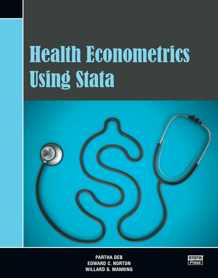
Health Econometrics Using Stata by Partha Deb, Edward C. Norton, and Willard G. Manning provides an excellent overview of the methods used to analyze data on healthcare expenditure and use. Aimed at researchers, graduate students, and practitioners, this book introduces readers to widely used methods, shows them how to perform these methods in Stata, and illustrates how to interpret the results. Each method is discussed in the context of an example using an extract from the Medical Expenditure Panel Survey.
After the overview chapters, the book provides excellent introductions to a series of topics aimed specifically at those analyzing healthcare expenditure and use data. The basic topics of linear regression, the generalized linear model, and log and Box-Cox models are covered with a tight focus on the problems presented by these data. Using this foundation, the authors cover the more advanced topics of models for continuous outcome with mass points, count models, and models for heterogeneous effects. Finally, they discuss endogeneity and how to address inference questions using data from complex surveys.
The authors use their formidable experience to guide readers toward useful methods and away from less recommended ones. Their discussion of "health econometric myths" and the chapter presenting a framework for approaching health econometric estimation problems are especially useful for this aspect.
Partha Deb is a professor of economics at Hunter College, City University of New York, where he teaches econometrics at the undergraduate and graduate levels. He has also taught, like his coauthors of this book, short courses in econometrics in the US, Europe, and Australia. He has developed a number of modeling packages in Stata. His research spans a range of topics that involve development and application of novel econometric methods in health economics, including modeling healthcare expenditures and use.
Edward C. Norton is an economist at the University of Michigan, where he is a professor in the Department of Health Management and Policy and in the Department of Economics. His research interests in health economics include long-term care and aging, obesity, pay for performance, and applied econometrics. He is an associate editor for both Health Economics and the Journal of Health Economics. He has taught econometrics at the doctoral and master’s levels, making extensive use of Stata, for many years.
Willard G. Manning was a professor at the Harris School and Health Studies at the University of Chicago at the time of his death in 2014. He had previously held positions at the University of Minnesota, University of Michigan, UCLA, RAND Corporation, and Harvard. He was well known as a champion of developing and applying rigorous econometric methods in health economics during his long career.
1.2 Themes
1.3 Health econometric myths
1.4 Stata friendly
1.5 A useful way forward
2.2 Potential outcomes and treatment effects
2.3 Estimating ATEs
2.3.2 Randomization
2.3.3 Covariate adjustment
2.4.2 Nonlinear regression
2.6 Model selection
2.6.2 Cross-validation
3.2 Overview of all variables
3.3 Expenditure and use variables
3.4 Explanatory variables
3.5 Sample dataset
3.6 Stata resources
4.2 The linear regression model
4.3 Marginal, incremental, and treatment effects
4.3.2 Graphical representation of marginal and incremental effects
4.3.3 Treatment effects
4.4.2 Example: An exponential specification
4.5.2 MEPS example of visual checks
4.6.2 Ramsey's RESET test
4.6.3 Modified Hosmer–Lemeshow test
4.6.4 Examples
4.6.5 Model selection using AIC and BIC
5.2 GLM framework
5.2.2 Parameter estimation
5.4 GLM predictions
5.5 GLM example with interaction term
5.6 Marginal and incremental effects
5.7 Example of marginal and incremental effects
5.8 Choice of link function and distribution family
5.8.2 Test for the link function
5.8.3 Modified Park test for the distribution family
5.8.4 Extended GLM
5.10 Stata resources
6.2 Log models
6.3.2 Marginal and incremental effects
6.5 Box–Cox models
7.2 Two-part models
7.5.2 Two-part model marginal effects
7.5.3 Two-part model marginal effects example
7.5.4 Generalized tobit interpretation
7.5.5 Generalized tobit example
7.6.2 Why tobit is used sparingly
7.6.3 One-part models
7.8 Stata resources
8.2 Poisson regression
8.2.2 Robustness of the Poisson regression
8.2.3 Interpretation
8.2.4 Is Poisson too restrictive?
8.4.2 Zero-inflated models
8.5.2 Censoring
8.6.2 Cross-validation
8.8 Stata resources
9.2 Quantile regression
9.2.2 Extensions
9.3.2 MEPS example of healthcare use
9.6 Stata resources
10.2 Endogeneity in linear models
10.2.2 2SLS
10.2.3 Specification tests
10.2.4 2SRI
10.2.5 Modeling endogeneity with ERM
10.5 Stata resources
11.2 Features of sampling designs
11.2.2 Clusters and stratification
11.2.3 Weights and clustering in natural experiments
11.3.2 Standard errors
11.4.2 Weighted sample means
11.4.3 Weighted least-squares regression
11.4.4 Weighted Poisson count model
11.6 Stata resources


