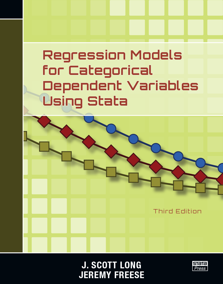
Regression Models for Categorical Dependent Variables Using Stata, Third Edition
121,000원
Authors: J. Scott Long and Jeremy Freese Publisher: Stata Press Copyright: 2014 ISBN-13: 978-1-59718-111-2 Pages: 589; paperback
Regression Models for Categorical Dependent Variables Using Stata, Third Edition, by J. Scott Long and Jeremy Freese, is an essential reference for those who use Stata to fit and interpret regression models for categorical data. Although regression models for categorical dependent variables are common, few texts explain how to interpret such models; this text decisively fills the void.
The third edition is divided into two parts. Part I begins with an excellent introduction to Stata and follows with general treatments of the estimation, testing, fitting, and interpretation of models for categorical dependent variables. The book is thus accessible to new users of Stata and those who are new to categorical data analysis. Part II is devoted to a comprehensive treatment of estimation and interpretation for binary, ordinal, nominal, and count outcomes.
Readers familiar with previous editions will find many changes in the third edition. An entire chapter is now devoted to interpretation of regression models using predictions. This concept is explored in greater depth in Part II. The authors also discuss how many improvements made to Stata in recent years—factor variables, marginal effects with margins, plotting predictions using marginsplot—facilitate analysis of categorical data.
The authors advocate a variety of new methods that use predictions to interpret the effect of variables in regression models. Readers will find all discussion of statistical concepts firmly grounded in concrete examples. All the examples, datasets, and author-written commands are available on the authors' website, so readers can easily replicate the examples with Stata.
Examples in the new edition also illustrate changes to the authors' popular SPost commands after a recent rewrite inspired by the authors' evolving views on interpretation. Readers will note that SPost now takes full advantage of the power of the margins command and the flexibility of factor-variable notation. Long and Freese also provide a suite of new commands, including mchange, mtable, and mgen. These commands complement margins, aiding model interpretation, hypothesis testing, and model diagnostics. They offer the same syntactical convenience features that users of Stata expect, for example including powers or interactions of covariates in regression models and seamlessly working with complex survey data. The authors also discuss how to use these commands to estimate marginal effects, either averaged over the sample or evaluated at fixed values of the regressors.
The third edition of Regression Models for Categorical Dependent Variables Using Stata continues to provide the same high-quality, practical tutorials of previous editions. It also offers significant improvements over previous editions—new content, updated information about Stata, and updates to the authors' own commands. This book should be on the bookshelf of every applied researcher analyzing categorical data and is an invaluable learning resource for students and others who are new to categorical data analysis.
Scott Long is Distinguished Professor of Sociology and Statistics at Indiana University–Bloomington. He has contributed articles to many journals, including the American Sociological Review, American Journal of Sociology, American Statistician, and Sociological Methods and Research. Dr. Long has authored or edited seven previous books on statistics, including the highly acclaimed Regression Models for Categorical and Limited Dependent Variables and The Workflow of Data Analysis Using Stata. In 2001, he received the Paul Lazarsfeld Memorial Award for Distinguished Contributions to Sociological Methodology. He is an elected Fellow of the American Statistical Association and a member of the Sociological Research Association.
Jeremy Freese is Ethel and John Lindgren Professor of Sociology and Faculty Fellow of the Institute for Policy Research at Northwestern University. He has previously been a faculty member at the University of Wisconsin–Madison and a Robert Wood Johnson Scholar in Health Policy Research at Harvard University. He has published numerous research articles in journals, including the American Sociological Review, American Journal of Sociology, and Public Opinion Quarterly. He has also taught categorical data analysis at the ICPSR Summer Program in Quantitative Methods and at El Colegio de México.
1.2 Which models are considered?
1.3 Whom is this book for?
1.4 How is the book organized?
1.5 The SPost software
1.5.2 Installing SPost13
Installing SPost13 using search
Installing SPost13 using net install
1.6.2 Using spex to load data and run examples
1.7.2 Getting help from the authors
2.2 Abbreviations
2.3 Getting help
2.3.2 PDF manuals
2.3.3 Error messages
2.3.4 Asking for help
2.3.5 Other resources
2.5 Stata file types
2.6 Saving output to log files
2.7 Using and saving datasets
2.7.2 Data in other formats
2.7.3 Entering data by hand
2.9 Do-files
2.9.2 Long lines
2.9.3 Stopping a do-file while it is running
2.9.4 Creating do-files
2.9.5 Recommended structure for do-files
2.11 Syntax of Stata commands
2.11.2 Variable lists
2.11.3 if and in qualifiers
2.11.4 Options
2.12.2 Getting information about variables
2.12.3 Missing values
2.12.4 Selecting observations
2.12.5 Selecting variables
2.13.2 The replace command
2.13.3 The recode command
2.14.2 Value labels
2.14.3 The notes command
2.16 Loops using foreach and forvalues
2.17 Graphics
2.19 A do-file template
2.20 Conclusion
3.1.2 ML and sample size
3.1.3 Problems in obtaining ML estimates
3.1.4 Syntax of estimation commands
3.1.5 Variable lists
Specifying interaction and polynomials
More on factor-variable notation
Information about missing values
Postestimation commands and the estimation sample
3.1.9 Robust standard errors
3.1.10 Reading the estimation output
3.1.11 Storing estimation results
3.2.2 Wald and likelihood-ratio tests
3.2.3 Wald tests with test and testparm
3.2.4 LR tests with lrtest
3.3.2 Methods and formulas used by fitstat
3.3.3 Example of fitstat
3.5 Conclusion
4.2 Approaches to interpretation
4.2.2 Method of interpretation using parameters
4.2.3 Stata and SPost commands for interpretation
4.4 Predictions at specified values
4.4.2 Using margins for predictions
Making multiple predictions
Predictions for groups defined by levels of categorical variables
The expression() option
(Advanced) Combining and formatting tables using mtable
4.5.2 Marginal effects using mtable
4.5.3 Posting predictions and using mlincom
4.5.4 Marginal effects using mchange
4.6.2 Plotting predictions using mgen
4.7.2 Standardized coefficients
4.7.3 Factor and percentage change coefficients
5.1.2 A nonlinear probability model
5.2.2 Comparing logit and probit
5.2.3 (Advanced) Observations predicted perfectly
5.3.2 Testing multiple coefficients
5.3.3 Comparing LR and Wald tests
5.4.2 Residuals and influential observations using predict
5.4.3 Least likely observations
5.5.2 Pseudo-R²'s
5.5.3 (Advanced) Hosmer–Lemeshow statistic
5.7 Conclusion
6.1.2 (Advanced) Interpretation using y*
6.2.2 Summary measures of change
AMEs
Standard errors of marginal effects
6.2.4 Examples of marginal effects
AMEs for factor variables
Summary table of AMEs
Marginal effects for subgroups
MEMs and MERs
Marginal effects with powers and interactions
6.2.6 (Advanced) Algorithm for computing the distribution of effects
6.3.2 Comparing ideal types with statistical tests
6.3.3 (Advanced) Using macros to test differences between ideal types
6.3.4 Marginal effects for ideal types
6.5 Second differences comparing marginal effects
6.6. Graphing predicted probabilities
6.6.2 Using mgen with the graph command
6.6.3 Graphing multiple predictions
6.6.4 Overlapping confidence intervals
6.6.5 Adding power terms and plotting predictions
6.6.6 (Advanced) Graphs with local means
7.1.2 A nonlinear probability model
7.2.2 Predicting perfectly
7.3.2 Testing multiple coefficients
7.5 (Advanced) Converting to a different parameterization
7.6 The parallel regression assumption
7.6.2 Testing the parallel regression assumption using brant
7.6.3 Caveat regarding the parallel regression assumption
7.8 Interpreting transformed coefficients
7.8.2 Odds ratios
7.10 Predicted probabilities with predict
7.11 Marginal effects
7.11.2 Marginal effects for a quick overview
7.14 Plotting predicted probabilities
7.15 Probability plots and marginal effects
7.16 Less common models for ordinal outcomes
7.16.2 The generalized ordered logit model
7.16.3 (Advanced) Predictions without using factor-variable notation
7.16.4 The sequential logit model
Options
8.2.2 Selecting different base outcomes
8.2.3 Predicting perfectly
8.3.2 Testing the effects of the independent variables
8.3.3 Tests for combining alternatives
8.4.2 Small-Hsiao test of IIA
8.6 Overview of interpretation
8.7 Predicted probabilities with predict
8.8 Marginal effects
8.9.2 (Advanced) Predictions using local means and subsamples
8.11 Odds ratios
8.11.2 Plotting odds ratios
8.12.2 Conditional logit model
8.12.3 Multinomial probit model with IIA
8.12.4 Alternative-specific multinomial probit
8.12.5 Rank-ordered logit model
9.1.2 Compaing observed and predicted counts with mgen
Treating a count independent variable as a factor variable
Predicted probabilities using mgen
9.2.6 (Advanced) Exposure time
9.3.3 Testing for overdispersion
9.3.4 Comparing the PRM and NBRM using estimates table
9.3.5 Robust standard errors
9.3.6 Interpretation using E(y | x)
9.3.7 Interpretation using predicted probabilities
9.4.3 Predictions in the estimation sample
9.4.4 Interpretation using predicted rates and probabilities
9.5.2 Predictions in the sample
9.5.3 Predictions at user-specified values
9.5.4 Warning regarding sample specification
9.6.2 Example of zero-inflated models
9.6.3 Interpretation of coefficients
9.6.4 Interpretation of predicted probabilities
Plotting predicted probabilities with mgen
9.7.2 Tests to compare count models
9.7.3 Using countfit to compare count models

