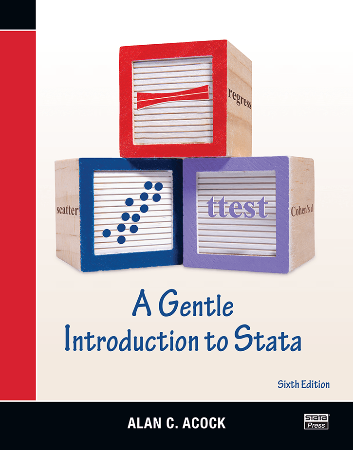
A Gentle Introduction to Stata, Sixth Edition
97,500원 80,000원
Author: Alan C. Acock Publisher: Stata Press Copyright: 2018 ISBN-13: 978-1-59718-269-0 Pages: 570; paperback
Alan C. Acock's A Gentle Introduction to Stata, Sixth Edition is aimed at new Stata users who want to become proficient in Stata. After reading this introductory text, new users will be able not only to use Stata well but also to learn new aspects of Stata.
Acock assumes that the user is not familiar with any statistical software. This assumption of a blank slate is central to the structure and contents of the book. Acock starts with the basics; for example, the part of the book that deals with data management begins with a careful and detailed example of turning survey data on paper into a Stata-ready dataset on the computer. When explaining how to go about basic exploratory statistical procedures, Acock includes notes that will help the reader develop good work habits. This mixture of explaining good Stata habits and good statistical habits continues throughout the book.
Acock is quite careful to teach the reader all aspects of using Stata. He covers data management, good work habits (including the use of basic do-files), basic exploratory statistics (including graphical displays), and analyses using the standard array of basic statistical tools (correlation, linear and logistic regression, and parametric and nonparametric tests of location and dispersion). He also successfully introduces some more advanced topics such as multiple imputation and multilevel modeling in a very approachable manner. Acock teaches Stata commands by using the menus and dialog boxes while still stressing the value of do-files. In this way, he ensures that all types of users can build good work habits. Each chapter has exercises that the motivated reader can use to reinforce the material.
The tone of the book is friendly and conversational without ever being glib or condescending. Important asides and notes about terminology are set off in boxes, which makes the text easy to read without any convoluted twists or forward referencing. Rather than splitting topics by their Stata implementation, Acock arranges the topics as they would appear in a basic statistics textbook; graphics and postestimation are woven into the material in a natural fashion. Real datasets, such as the General Social Surveys from 2002, 2006, and 2016, are used throughout the book.
The focus of the book is especially helpful for those in the behavioral and social sciences because the presentation of basic statistical modeling is supplemented with discussions of effect sizes and standardized coefficients. Various selection criteria, such as semipartial correlations, are discussed for model selection. Acock also covers a variety of commands available for evaluating reliability and validity of measurements.
The sixth edition incorporates new features of Stata 15. All menus, dialog boxes, and instructions for using the point-and-click interface have been updated. Power-and-sample-size calculations for linear regression are demonstrated using Stata 15's new power rsquared command. This edition also includes new sections that describe how to evaluate convergent and discriminant validity, how to compute effect sizes for t tests and ANOVA models, how to use margins and marginsplot to interpret results of linear and logistic regression models, and how to use full-information maximum-likelihood (FIML) estimation with SEM to address problems with missing data.
Alan Acock is a sociologist and a University Distinguished Professor Emeritus in the School of Social and Behavioral Health Sciences at Oregon State University. He held the Knudson Chair in Family Research and was also recognized as the Alumni Distinguished Professor based on his work with students. He is the author of Discovering Structural Equation Modeling Using Stata, Revised Edition. He has published more than 150 articles in leading journals across the social and behavioral sciences, including Structural Equation Modeling, Psychological Bulletin, Multivariate Behavioral Research, Journal of Gerontology, Journal of Adolescence, American Journal of Public Health, American Sociological Review, Journal of Marriage and Family, Social Forces, Drug and Alcohol Dependence, Educational and Psychological Measurement, Journal of Politics, Prevention Science, American Journal of Preventive Medicine, and many others. With this broad experience, Acock brings examples from a variety of disciplines.
1.2 Introduction
1.3 The Stata screen
1.4 Using an existing dataset
1.5 An example of a short Stata session
1.6 Video aids to learning Stata
1.7 Summary
1.8 Exercises
2.2 An example questionnaire
2.3 Developing a coding system
2.4 Entering data using the Data Editor
2.6 The Data Editor (Browse) view
2.7 Saving your dataset
2.8 Checking the data
2.9 Summary
2.10 Exercises
3.2 Planning your work
3.3 Creating value labels
3.4 Reverse-code variables
3.5 Creating and modifying variables
3.6 Creating scales
3.7 Saving some of your data
3.8 Summary
3.9 Exercises
4.2 How Stata commands are constructed
4.3 Creating a do-file
4.4 Copying your results to a word processor
4.5 Logging your command file
4.6 Summary
4.7 Exercises
5.2 Where is the center of a distribution?
5.3 How dispersed is the distribution?
5.4 Statistics and graphs—unordered categories
5.5 Statistics and graphs—ordered categories and variables
5.6 Statistics and graphs—quantitative variables
5.7 Summary
5.8 Exercises
6.2 Cross-tabulation
6.3 Chi-squared test
6.3.2 Probability tables
6.5 Odds ratios when dependent variable has two categories
6.6 Ordered categorical variables
6.7 Interactive tables
6.8 Tables—linking categorical and quantitative variables
6.9 Power analysis when using a chi-squared test of significance
6.10 Summary
6.11 Exercises
7.2 Randomization
7.3 Random sampling
7.4 Hypotheses
7.5 One-sample test of a proportion
7.6 Two-sample test of a proportion
7.7 One-sample test of means
7.8 Two-sample test of group means
7.10 Power analysis
7.11 Nonparametric alternatives
7.11.2 Nonparametric alternative: Median test
7.13 Summary
7.14 Exercises
8.2 Scattergrams
8.3 Plotting the regression line
8.4 An alternative to producing a scattergram, binscatter
8.5 Correlation
8.6 Regression
8.7 Spearman’s rho: Rank-order correlation for ordinal data
8.8 Power analysis with correlation
8.9 Summary
8.10 Exercises
9.2 ANOVA example
9.3 ANOVA example with nonexperimental data
9.4 Power analysis for one-way ANOVA
9.5 A nonparametric alternative to ANOVA
9.6 Analysis of covariance
9.7 Two-way ANOVA
9.8 Repeated-measures design
9.9 Intraclass correlation—measuring agreement
9.10 Power analysis with ANOVA
9.10.2 Power analysis for two-way ANOVA
9.10.3 Power analysis for repeated-measures ANOVA
9.10.4 Summary of power analysis for ANOVA
9.12 Exercises
10.2 What is multiple regression?
10.3 The basic multiple regression command
10.4 Increment in R-squared: Semipartial correlations
10.5 Is the dependent variable normally distributed?
10.6 Are the residuals normally distributed?
10.7 Regression diagnostic statistics
10.7.2 Influential observations: DFbeta
10.7.3 Combinations of variables may cause problems
10.9 Categorical predictors and hierarchical regression
10.10 A shortcut for working with a categorical variable
10.11 Fundamentals of interaction
10.12 Nonlinear relations
10.12.2 Centering when using a quadratic term
10.12.3 Do we need to add a quadratic component?
10.14 Summary
10.15 Exercises
11.2 An example
11.3 What is an odds ratio and a logit?
11.3.2 The logit transformation
11.5 Logistic regression
11.6 Hypothesis testing
11.6.2 Testing sets of coefficients
11.8 Nested logistic regressions
11.9 Power analysis when doing logistic regression
11.10 Next steps for using logistic regression and its extensions
11.11 Summary
11.12 Exercises
12.2 Constructing a scale
12.3.2 Equivalence
12.3.3 Split-half and alpha reliability—internal consistency
12.3.4 Kuder–Richardson reliability for dichotomous items
12.3.5 Rater agreement—kappa (κ)
12.4.2 Criterion-related validity
12.4.3 Construct validity
12.6 PCF analysis
12.6.2 Oblique rotation: Promax
12.9 Exercises
13.1.2 SEM and working with missing values
13.1.3 Exploring missing values and auxiliary variables
13.1.4 Getting auxiliary variables into your SEM command
13.3 The gsem command for logistic regression
13.3.2 Fitting the model using the gsem command
13.5 Conclusions and what is next for the sem command
13.6 Exercises
14.2 What variables do we include when doing imputations?
14.3 The nature of the problem
14.4 Multiple imputation and its assumptions about the mechanism for missingness
14.5 Multiple imputation
14.6 A detailed example
14.6.2 Setup and multiple-imputation stage
14.6.3 The analysis stage
14.6.4 For those who want an R2 and standardized βs
14.6.5 When impossible values are imputed
14.8 Exercises
15.2 Questions and data for a longitudinal multilevel application
15.3 Fixed-effects regression models
15.4 Random-effects regression models
15.5 An applied example
15.5.2 Reshaping data to do multilevel analysis
15.7 Random-intercept model
15.7.2 Random-intercept model—quadratic term
15.7.3 Treating time as a categorical variable
15.9 Including a time-invariant covariate
15.10 Summary
15.11 Exercises
16.2 Overview of three IRT models for dichotomous items
16.2.2 The two-parameter logistic (2PL) model
16.2.3 The three-parameter logistic (3PL) model
16.3.2 How important is each of the items?
16.3.3 An overall evaluation of our scale
16.3.4 Estimating the latent score
16.5.2 Fitting our graded response model
16.5.3 Estimating a person’s score
16.7 Using the Stata menu system
16.8 Extensions of IRT
16.9 Exercises
A.2 Resources
A.2.2 Books about Stata
A.2.3 Short courses
A.2.4 Acquiring data
A.2.5 Learning from the postestimation methods


