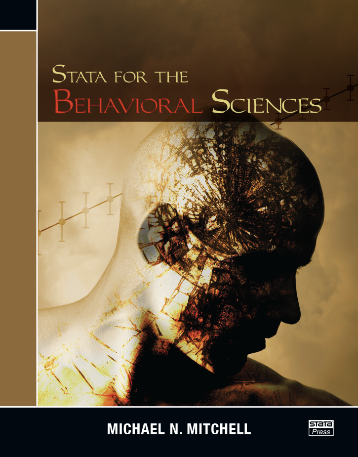
Stata for the Behavioral Sciences
121,000원
Author: Michael N. Mitchell Publisher: Stata Press Copyright: 2015 ISBN-13: 978-1-59718-173-0 Pages: 646; paperback
Stata for the Behavioral Sciences, by Michael Mitchell, is the ideal reference for researchers using Stata to fit ANOVA models and other models commonly applied to behavioral science data. Drawing on his education in psychology and his experience in consulting, Mitchell uses terminology and examples familiar to the reader as he demonstrates how to fit a variety of models, how to interpret results, how to understand simple and interaction effects, and how to explore results graphically.
Although this book is not designed as an introduction to Stata, it is appealing even to Stata novices. Throughout the text, Mitchell thoughtfully addresses any features of Stata that are important to understand for the analysis at hand. He also is careful to point out additional resources such as related videos from Stata's YouTube channel.
The book is divided into five sections.
The first section contains a chapter that introduces Stata commands for descriptive statistics and another that covers basic inferential statistics such as one- and two-sample t tests.
The second section focuses on between-subjects ANOVA modeling. The discussion moves from one-way ANOVA models to ANCOVA models to two-way and three-way ANOVA models. In each case, special attention is given to the use of commands such as contrast and margins for testing specific hypotheses of interest. Mitchell also emphasizes the understanding of interactions through contrasts and graphs. Underscoring the importance of planning any experiment, he discusses power analysis for t tests, for one- and two-way ANOVA models, and for ANCOVA models.
Section three of the book extends the discussion in the previous section to models for repeated-measures data and for longitudinal data.
The fourth section of the book illustrates the use of the regress command for fitting multiple regression models. Mitchell then turns his attention to tools for formatting regression output, for testing assumptions, and for model building. This section ends with a discussion of power analysis for simple, multiple, and nested regression models.
The final section has a tone that differs from the first four. Rather than focusing on a particular type of analysis, Mitchell describes elements of Stata. He first discusses estimation commands and similarities in syntax from command to command. Then, he details a set of postestimation commands that are available after most estimation commands. Another chapter provides an overview of data management commands. This section ends with a chapter that will be of particular interest to anyone who has used IBM® SPSS®; it lists commonly used SPSS® commands and provides equivalent Stata syntax.
This book is an easy-to-follow guide to analyzing data using Stata for researchers in the behavioral sciences and a valuable addition to the bookshelf of anyone interested in applying ANOVA methods to a variety of experimental designs.
Michael Mitchell is a senior statistician working in the area of sleep research as well as the prevention of child maltreatment. He is the author of A Visual Guide to Stata Graphics, Data Management Using Stata, and Interpreting and Visualizing Regression Models Using Stata. Previously, he worked for 12 years as a statistical consultant and manager of the UCLA ATS Statistical Consulting Group. There he envisioned the UCLA Statistical Consulting Resources website and wrote hundreds of webpages about Stata.
1.1.2 Other user-written programs
The esttab command
The extremes command
1.2.2 Supercharging your ANOVA
1.2.3 Stata is economical
1.2.4 Statistical powerhouse
1.2.5 Easy to learn
1.2.6 Simple and powerful data management
1.2.7 Access to user-written programs
1.2.8 Point and click or commands: Your choice
1.2.9 Powerful yet simple
1.2.10 Access to Stata source code
1.2.11 Online resources for learning Stata
1.2.12 And yet there is more!
1.3.2 Part II: Between-subjects ANOVA models
1.3.3 Part III: Repeated measures and longitudinal models
1.3.4 Part IV: Regression models
1.3.5 Part V: Stata overview
1.3.6 The GSS dataset
1.3.7 Language used in the book
1.3.8 Online resources for this book
1.4.2 Data management in Stata
1.4.3 Reproducing your results
1.4.4 Recommended Stata Press books
2.2 Using and describing the GSS dataset
2.3 One-way tabulations
2.4 Summary statistics
2.5 Summary statistics by one group
2.6 Two-way tabulations
2.7 Cross-tabulations with summary statistics
2.8 Closing thoughts
3.2 Two-sample t tests
3.3 Paired sample t tests
3.4 One-sample t tests
3.5 Two-sample test of proportions
3.6 One-sample test of proportions
3.7 Chi-squared and Fisher's exact test
3.8 Correlations
3.9 Immediate commands
3.9.2 Immediate test of one mean
3.9.3 Immediate test of two proportions
3.9.4 Immediate test of one proportion
3.9.5 Immediate cross-tabulations
4.2 Comparing two groups using a t test
4.3 Comparing two groups using ANOVA
4.4.2 Computing effect sizes for planned comparisons
4.6 Interpreting confidence intervals
4.7 Closing thoughts
5.2 Introducing contrasts
5.2.2 Making contrasts among means
5.2.3 Graphing contrasts
5.2.4 Options with the margins and contrast commands
5.2.5 Computing effect sizes for contrasts
5.2.6 Summary
5.4 Compare each group against a reference group
5.4.2 Selecting a different reference group
5.4.3 Selecting a contrast and reference group
5.6.2 Selecting a specific contrast
5.7.2 Selecting a specific contrast
5.9 Custom contrasts
5.10 Weighted contrasts
5.11 Pairwise comparisons
5.12 Closing thoughts
6.2 Example 1: ANCOVA with an experiment using a pretest
6.3 Example 2: Experiment using covariates
6.4 Example 3: Observational data
6.4.2 Model 2: Demographics as covariates
6.4.3 Model 3: Demographics, socializing as covariates
6.4.4 Model 4: Demographics, socializing, health as covariates
6.5.2 Computing adjusted means: Method 2
6.5.3 Computing adjusted means: Method 3
6.5.4 Differences between method 2 and method 3
6.5.5 Adjusted means: Summary
7.2 Two-by-two models: Example 1
7.2.2 Estimating the size of the interaction
7.2.3 More about interaction
7.2.4 Summary
Simple contrasts
Partial interaction
Comparing optimism therapy with traditional therapy
Partial interactions
7.4.2 Simple contrasts
7.4.3 Partial interaction
7.4.4 Interaction contrasts
7.4.5 Summary
7.6 Interpreting confidence intervals
7.7 Closing thoughts
8.2 Example 1: IV has two levels
8.2.2 Question 2: When is optimism therapy superior?
8.2.3 Example 1: Summary
Question 1b
Question 2b
8.3.4 Example 2: Summary
9.2 Two-by-two-by-two models
9.2.2 Simple interactions by depression status
9.2.3 Simple effects
9.3.2 Simple partial interaction by depression status
9.3.3 Simple contrasts
9.3.4 Partial interactions
9.4.2 Simple interactions
9.4.3 Simple effects and simple contrasts
10.2 Performing ANOVA tests via regression
10.3 Supercharging your ANOVA
10.3.2 Homogeneity of variance
10.3.3 Robust regression
10.3.4 Quantile regression
10.5 Closing thoughts
11.2 Power analysis for a two-sample t test
11.2.2 Example 2: Using standardized effect sizes
11.2.3 Estimating effect sizes
11.2.4 Example 3: Power for a medium effect
11.2.5 Example 4: Power for a range of effect sizes
11.2.6 Example 5: For a given N, compute the effect size
11.2.7 Example 6: Compute effect sizes given unequal Ns
Hypothesis 2: Optimism therapy versus control
Hypothesis 3: Optimism therapy versus traditional therapy Summary of hypotheses
11.3.3 Example 8: Testing hypotheses 2 and 3
11.3.4 Summary
11.4.2 Example 10: Using correlated variables as covariates
11.5.2 Example 12: Standardized simple effects
11.5.3 Example 13: Standardized interaction effect
11.5.4 Summary: Power for two-way ANOVA
12.2 Example 1: One-way within-subjects designs
12.3 Example 2: Mixed design with two groups
12.4 Example 3: Mixed design with three groups
12.5 Comparing models with different residual covariance structures
12.6 Example 1 revisited: Using compound symmetry
12.7 Example 1 revisited again: Using small-sample methods
12.8 An alternative analysis: ANCOVA
12.9 Closing thoughts
13.2 Example 1: Linear effect of time
13.3 Example 2: Interacting time with a between-subjects IV
13.4 Example 3: Piecewise modeling of time
13.5 Example 4: Piecewise effects of time by a categorical predictor
13.5.2 Treatment slopes
13.5.3 Jump at treatment
13.5.4 Comparisons among groups at particular days
13.5.5 Summary of example 4
14.2 Simple linear regression
14.2.2 Computing predicted means using the margins command
14.2.3 Graphing predicted means using the marginsplot command
14.3.2 Running the multiple regression model
14.3.3 Computing adjusted means using the margins command
14.3.4 Describing the contribution of a predictor
Multiple-unit change
Milestone change in units
One SD change in predictor
Partial and semipartial correlation
14.4.2 Testing the equality of coefficients
14.4.3 Testing linear combinations of coefficients
15.2 Regression options
15.3 Redisplaying results
15.4 Identifying the estimation sample
15.5 Stored results
15.6 Storing results
15.7 Displaying results with the estimates table command
15.8 Closing thoughts
16.2 Presenting a single model
16.3 Presenting multiple models
16.4 Creating regression tables using esttab
16.4.2 Presenting multiple models with esttab
16.4.3 Exporting results to other file formats
16.5.2 outreg2
16.5.3 xml_tab
16.5.4 coefplot
17.2 Fitting multiple models on the same sample
17.3 Nested models
17.3.2 Example 2: A more realistic example
17.5 Closing thoughts
18.2 Outliers
18.2.2 Studentized residuals, leverage, Cook's D
18.2.3 Graphs of residuals, leverage, and Cook's D
18.2.4 DFBETAs and avplots
18.2.5 Running a regression with and without observations
18.3.2 Using scatterplots to check for nonlinearity
18.3.3 Checking for nonlinearity using residuals
18.3.4 Checking for nonlinearity using a locally weighted smoother
18.3.5 Graphing an outcome mean at each level of predictor
18.3.6 Summary
18.3.7 Checking for nonlinearity analytically
Using factor variables
18.5 Homoskedasticity
18.6 Normality of residuals
18.7 Closing thoughts
19.2 Power for simple regression
19.3 Power for multiple regression
19.4 Power for a nested multiple regression
19.5 Closing thoughts
20.2 Common syntax
20.3 Analysis using subsamples
20.4 Robust standard errors
20.5 Prefix commands
20.5.2 The nestreg: prefix
20.5.3 The stepwise: prefix
20.5.4 The svy: prefix
20.5.5 The mi estimate: prefix
20.7 Postestimation commands
20.8 Closing thoughts
21.2 The contrast command
21.3 The margins command
21.3.2 Margins with factor variables
21.3.3 Margins with factor variables and the at() option
21.3.4 The dydx() option
21.5 The pwcompare command
21.6 Closing thoughts
22.2 Reading data into Stata
22.2.2 Reading Excel workbooks
22.2.3 Reading comma-separated files
22.2.4 Reading other file formats
22.4 Labeling data
22.4.2 A looping trick
22.4.3 Value labels
22.5.2 Modifying existing variables with replace
22.5.3 Extensions to generate egen
22.5.4 Recode
22.7 Keeping and dropping observations
22.8 Combining datasets
22.8.2 Merging datasets
22.9.2 Reshaping datasets long to wide
23.2 ADD FILES
23.3 AGGREGATE
23.4 ANOVA
23.5 AUTORECODE
23.6 CASESTOVARS
23.7 COMPUTE
23.8 CORRELATIONS
23.9 CROSSTABS
23.10 DATA LIST
23.11 DELETE VARIABLES
23.12 DESCRIPTIVES
23.13 DISPLAY
23.14 DOCUMENT
23.15 FACTOR
23.16 FILTER
23.17 FORMATS
23.18 FREQUENCIES
23.19 GET FILE
23.20 GET TRANSLATE
23.21 LOGISTIC REGRESSION
23.22 MATCH FILES
23.23 MEANS
23.24 MISSING VALUES
23.25 MIXED
23.26 MULTIPLE IMPUTATION
23.27 NOMREG
23.28 PLUM
23.29 PROBIT
23.30 RECODE
23.31 RELIABILITY
23.32 RENAME VARIABLES
23.33 SAVE
23.34 SELECT IF
23.35 SAVE TRANSLATE
23.36 SORT CASES
23.37 SORT VARIABLES
23.38 SUMMARIZE
23.39 T-TEST
23.40 VALUE LABELS
23.41 VARIABLE LABELS
23.42 VARSTOCASES
23.43 Closing thoughts


