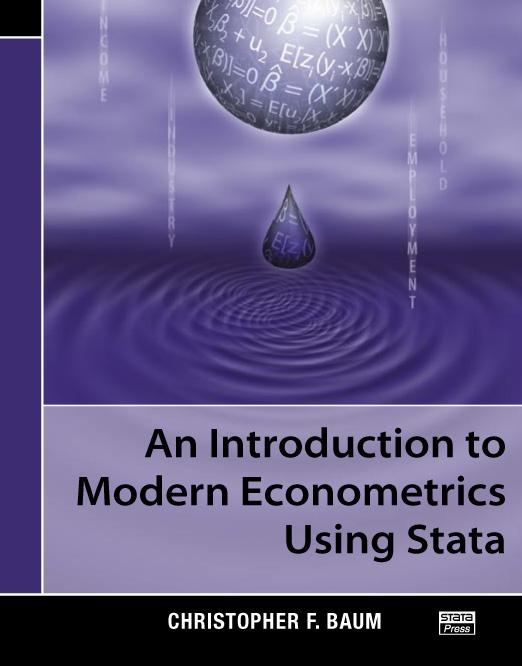
An Introduction to Modern Econometrics Using Stata
106,000원
Author: Christopher F. Baum Publisher: Stata Press Copyright: 2006 ISBN-13: 978-1-59718-013-9 Pages: 341; paperback
Author index
Subject index
Errata
Download the datasets used in this book
Review from the Stata Journal
Chinese and Russian translations available
An Introduction to Modern Econometrics Using Stata, by Christopher F. Baum, successfully bridges the gap between learning econometrics and learning how to use Stata. The book presents a contemporary approach to econometrics, emphasizing the role of method-of-moments estimators, hypothesis testing, and specification analysis while providing practical examples showing how the theory is applied to real datasets by using Stata.
The first three chapters are dedicated to the basic skills needed to effectively use Stata: loading data into Stata; using commands like generate and replace, egen, and sort to manipulate variables; taking advantage of loops to automate tasks; and creating new datasets by using merge and append. Baum succinctly yet thoroughly covers the elements of Stata that a user must learn to become proficient, providing many examples along the way.
Chapter 4 begins the core econometric material of the book and covers the multiple linear regression model, including efficiency of the ordinary least-squares estimator, interpreting the output from regress, and point and interval prediction. The chapter covers both linear and nonlinear Wald tests, as well as constrained least-squares estimation, Lagrange multiplier tests, and hypothesis testing of nonnested models.
Chapters 5 and 6 focus on consequences of failures of the linear regression model’s assumptions. Chapter 5 addresses topics like omitted-variable bias, misspecification of functional form, and outlier detection. Chapter 6 is dedicated to non-independently and identically distributed errors, and it introduces the Newey–West and Huber/White covariance matrices, as well as feasible generalized least-squares estimation in the presence of heteroskedasticity or serial correlation. Chapter 7 is dedicated to the use of indicator variables and interaction effects.
Instrumental-variables estimation has been an active area of research in econometrics, and chapter 8 commendably addresses issues like weak instruments, underidentification, and generalized method-of-moments estimation. In this chapter, Baum extensively uses his wildly popular ivreg2command.
The last two chapters briefly introduce panel-data analysis and discrete and limited-dependent variables. Two appendices detail importing data into Stata and Stata programming. As in all chapters, Baum presents many Stata examples.
An Introduction to Modern Econometrics Using Stata can serve as a supplementary text in both undergraduate- and graduate-level econometrics courses, and the book’s examples will help students quickly become proficient in Stata. The book is also useful to economists and businesspeople wanting to learn Stata by using practical examples.
Comments from readers
This book provides an excellent resource for both teaching and learning modern microeconometric practice, using the most popular software package in this area. The coverage includes discrete choice models and models for panel data, as well as linear regression and instrumental variables methods. I particularly like the material on handling large datasets and developing efficient programs within Stata, which provide the reader with an invaluable introduction to good practice in empirical research.
Prof. Steve Bond
Nuffield College, Oxford
and Institute for Fiscal Studies (IFS) London
Kit Baum provides students and researchers a hands-on guide to modern econometric techniques by means of many well-documented examples in Stata. The examples are also useful templates for those who need to write Stata routines for their own work. Treatment and transformation of cross-section, time-series, and panel data are carefully explained. The coverage of the text is broad and up to date. An Introduction to Modern Econometrics Using Stata is a valuable companion to undergraduate- and graduate-level econometric textbooks.
Serena Ng
Department of Economics, University of Michigan
Christopher Baum’s An Introduction to Modern Econometrics Using Stata is probably the only econometrics text published to date that pays serious attention to reproducibility of research and systematic data validation using Stata’s data audit commands along with do-file and programming capabilities. Economic and financial consultants will find this text to be an invaluable guide to using Stata for creating reproducible, error-free data and econometric analysis, as well as quality graphic presentations. The book is comprehensive and easy to follow, with substantive coverage of econometric theory and applications using the full array of Stata’s capabilities. This text should serve as an excellent learning and reference guide for every consultant.
Zaur Rzakhanov, Ph.D.
Associate, Analysis Group Inc.
Boston, Massachusetts
This book is a wonderful complement to the Stata technical manuals. It provides a wealth of practical tips and sample applications that help the intermediate-level Stata user advance in making the most efficient use of Stata. It is thoughtfully organized along the lines of an econometrics textbook, allowing practitioners to find relevant and useful commands, procedures, and examples by topics that are familiar and immediate. It also includes a most helpful appendix for novice programmers that will expedite their development into proficient Stata programmers. This book is a must-have reference for any organization that needs to train practitioners of econometrics in the use of Stata.
Peter Boberg
CRA International
For too long there has been a hole in the field between econometrics textbooks, which focus on theory but give little practical guidance to the day-to-day realities of economic research, and software manuals, which provide detail but little analytical context. Researchers, analysts, and students have no single source to turn to and often waste valuable time and effort reinventing the wheel. This book brings it all together and gives the researcher a huge step up on the learning curve. It perhaps should have been subtitled “How to perform high-quality empirical research using Stata.” It addresses topics in the order that real-world research is performed, beginning with the data-management and quality-control issues that a researcher must contend with every day and then proceeding to the econometric tools used for most empirical analyses. A researcher or a research analyst reading this book would learn insights and tricks of the trade that would otherwise take years to accumulate. Common errors (such as those resulting from many-to-many merges) are pointed out. Useful tips (such as the use of local macros) are discussed. Efficient and robust programming is encouraged throughout. This book should be required reading for any empirical researcher or research analyst interested in developing a high-quality research process.
Dr. Paul Liu
The Brattle Group
Christopher F. Baum is an economist at Boston College, where he codirects the undergraduate minor in scientific computation. He is an associate editor of the Stata Journal and co-organizer of Stata Users Group meetings in Boston. Baum has coauthored many Stata routines and maintains the Statistical Software Components archive of downloadable Stata packages. He has taught econometrics at the undergraduate and graduate levels, making extensive use of Stata, for many years.
1.2 Installing the necessary software
1.3 Installing the support materials
2.1.2 Variable types
2.1.3 _n and _N
2.1.4 generate and replace
2.1.5 sort and gsort
2.1.6 if exp and in range
2.1.7 Using if exp with indicator variables
2.1.8 Using if exp versus by varlist: with statistical commands
2.1.9 Labels and notes
2.1.10 The varlist
2.1.11 drop and keep
2.1.12 rename and renvars
2.1.13 The save command
2.1.14 insheet and infile
2.2.2 Recoding discrete and continuous variables
2.2.3 Handling missing data
2.2.5 Handling dates
2.2.6 Some useful functions for generate or replace
2.2.7 The egen command
egen functions from the user community
2.2.9 Local macros
2.2.10 Looping over variables: forvalues and foreach
2.2.11 Scalars and matrices
2.2.12 Command syntax and return values
3.2 Time-series data
3.4 Panel data
3.5.2 Other transforms of panel data
3.5.3 Moving-window summary statistics and correlations
3.7 Creating long-format datasets with append
3.7.2 The dangers of many-to-many merges
3.9.2 Data validation: assert and duplicates
4.2 Computing linear regression estimates
4.2.2 The sampling distribution of regression estimates
4.2.3 Efficiency of the regression estimator
4.2.4 Numerical identification of the regression estimates
4.3.2 The ANOVA table: ANOVA F and R-squared
4.3.3 Adjusted R-squared
4.3.4 The coefficient estimates and beta coefficients
4.3.5 Regression without a constant term
4.3.6 Recovering estimation results
4.3.7 Detecting collinearity in regression
4.5.2 Wald tests involving linear combinations of parameters
4.5.3 Joint hypothesis tests
4.5.4 Testing nonlinear restrictions and forming nonlinear combinations
4.5.5 Testing competing (nonnested) models
4.A Appendix: Regression as a least-squares estimator
4.B Appendix: The large-sample VCE for linear regression
5.2 Specification error
5.2.3 Added-variable plots
5.2.4 Including irrelevant variables in the model
5.2.5 The asymmetry of specification error
5.2.6 Misspecification of the functional form
5.2.7 Ramsey's RESET
5.2.8 Specification plots
5.2.9 Specification and interaction terms
5.2.10 Outlier statistics and measures of leverage
The DFBETA statistic
6.1.2 The robust estimator of VCE
6.1.3 The cluster estimator of VCE
6.1.4 The Newey–West estimator of VCE
6.1.5 The generalized-least squares estimator
FGLS estimation
FGLS estimation
6.3.2 FGLS estimation with serial correlation
7.1.2 Regression with two qualitative measures
7.4 Testing for structural stability and structural change
7.4.2 Structural change in a time-series model
8.2 Endogeneity in economic relationships
8.3 2SLS
8.4 The ivreg command
8.5 Identification and tests of overidentifying restrictions
8.6 Computing IV estimates 8.7 ivreg2 and GMM estimation
8.7.2 GMM in a homoskedastic context
8.7.3 GMM and heteroskedasticity-consistent standard errors
8.7.4 GMM and clustering
8.7.5 GMM and HAC standard errors
8.10 Testing the relevance of instruments
8.11 Durbin–Wu–Hausman tests for endogeneity in IV estimation
8.A Appendix: Omitted-variables bias
8.B Appendix: Measurement error
9.1.2 Time effects and two-way FE
9.1.3 The between estimator
9.1.4 One-way RE
9.1.5 Testing the appropriateness of RE
9.1.6 Prediction from one-way FE and RE
9.3 Dynamic panel-data models
9.4 Seemingly unrelated regression models
10.1.2 Marginal effects and predictions
Binomial logit and grouped logit
10.3 Truncated regression and tobit models
10.3.2 Censoring
10.5 Bivariate probit and probit with selection
The insheet command
A.1.3 Fixed-format data files
B.1.2 Extended macro functions and list functions
B.3 Loop constructs
B.5 return and ereturn
B.7 Using Mata functions in Stata programs

