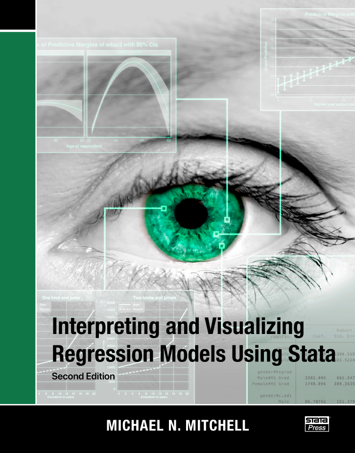
Interpreting and Visualizing Regression Models Using Stata, Second Edition

Michael Mitchell's Interpreting and Visualizing Regression Models Using Stata, Second Edition is a clear treatment of how to carefully present results from model-fitting in a wide variety of settings. It is a boon to anyone who has to present the tangible meaning of a complex model clearly, regardless of the audience. As an example, many experienced researchers start to squirm when asked to give a simple explanation of the practical meaning of interactions in nonlinear models such as logistic regression. The techniques presented in Mitchell's book make answering those questions easy. The overarching theme of the book is that graphs make interpreting even the most complicated models containing interaction terms, categorical variables, and other intricacies straightforward.

Using a dataset based on the General Social Survey, Mitchell starts with a basic linear regression with a single independent variable and then illustrates how to tabulate and graph predicted values. Mitchell focuses on Stata's margins and marginsplot commands, which play a central role in the book and which greatly simplify the calculation and presentation of results from regression models. In particular, through use of the marginsplot command, he shows how you can graphically visualize every model presented in the book and thus gain insight into results much easier when you can view them in a graph rather than in a mundane table of results.

Mitchell then proceeds to more complicated models where the effects of the independent variables are nonlinear. After discussing how to detect nonlinear effects, he presents examples using both standard polynomial models, where independent variables can be raised to powers like -1 or 1/2. In all cases, Mitchell again uses the marginsplot command to illustrate the effect that changing an independent variable has on the dependent variable. Piecewise linear models are presented as well; these are linear models in which the slope or intercept is allowed to change depending on the range of an independent variable. He also uses the contrast command when discussing categorical variables; as the name suggests, this command allows you to easily contrast predictions made for various levels of the categorical variable.

Interaction terms can be tricky to interpret, but Mitchell shows how graphs produced by marginsplot greatly clarify results. Individual chapters are devoted to two- and three-way interactions containing all continuous or all categorical variables and include many practical examples. Raw regression output including interactions of continuous and categorical variables can be nearly impossible to interpret, but again Mitchell makes this a snap through judicious use of the margins and marginsplot commands in subsequent chapters.

The first two-thirds of the book is devoted to cross-sectional data, while the final third considers longitudinal data and complex survey data. A significant difference between this book and most others on regression models is that Mitchell spends quite some time on fitting and visualizing discontinuous models--models where the outcome can change value suddenly at thresholds. Such models are natural in settings such as education and policy evaluation, where graduation or policy changes can make sudden changes in income or revenue.

The second edition has been updated to incorporate many new features added since Stata 12, when the first edition was written. Specifically, the text now demonstrates how labels on the values of categorical variables make interpretation much easier when looking at regression results and results from the margins and contrast commands. For instance, you now see that your coefficients or marginal means are related to the "low-dose" and "high-dose" groups instead of groups 1 and 2. In addition, Mitchell now shows you how to customize output from estimation commands, margins, and contrast for even more clarity. In his discussion of customizing graphs produced by marginsplot, he demonstrates new graph features such as the use of transparency. He also includes new examples of multilevel models for longitudinal data that take advantage of the degree-of-freedom adjustments for small sample sizes that are now provided by mixed and contrast.

This book is a worthwhile addition to the library of anyone involved in statistical consulting, teaching, or collaborative applied statistical environments. Graphs greatly aid the interpretation of regression models, and Mitchell's book shows you how.