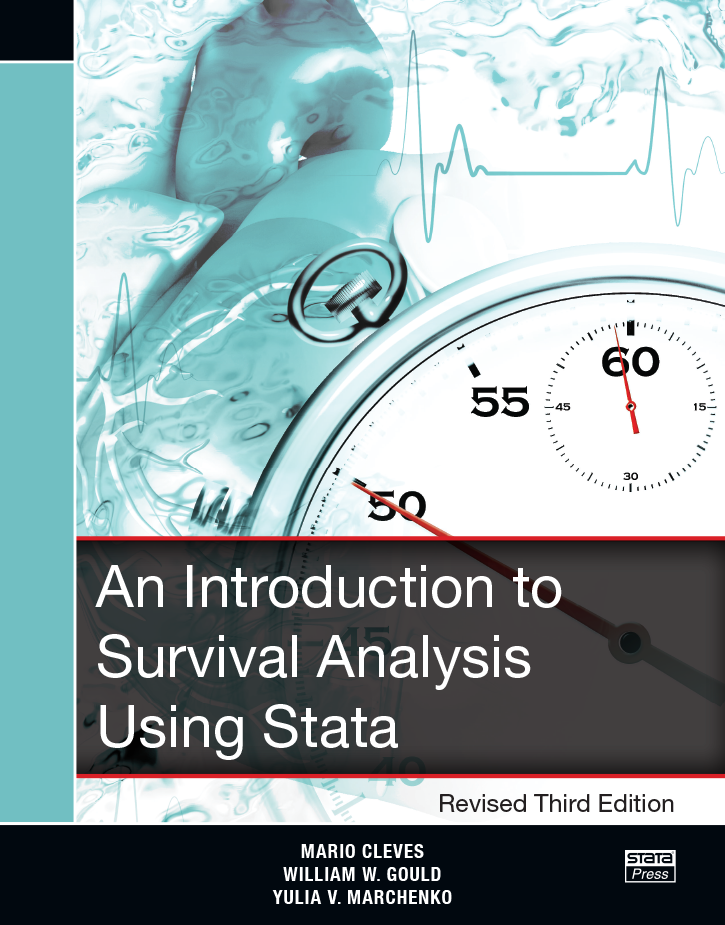
An Introduction to Survival Analysis Using Stata, Revised Third Edition
115,000원
Authors: Mario Cleves, William W. Gould, and Yulia V. Marchenko Publisher: Stata Press Copyright: 2016 ISBN-13: 978-1-59718-174-7 Pages: 428; paperback
An Introduction to Survival Analysis Using Stata, Revised Third Edition is the ideal tutorial for professional data analysts who want to learn survival analysis for the first time or who are well versed in survival analysis but are not as dexterous in using Stata to analyze survival data. This text also serves as a valuable reference to those readers who already have experience using Stata’s survival analysis routines.
The revised third edition has been updated for Stata 14, and it includes a new section on predictive margins and marginal effects, which demonstrates how to obtain and visualize marginal predictions and marginal effects using the margins and marginsplot commands after survival regression models.
Survival analysis is a field of its own that requires specialized data management and analysis procedures. To meet this requirement, Stata provides the st family of commands for organizing and summarizing survival data.
This book provides statistical theory, step-by-step procedures for analyzing survival data, an in-depth usage guide for Stata's most widely used stcommands, and a collection of tips for using Stata to analyze survival data and to present the results. This book develops from first principles the statistical concepts unique to survival data and assumes only a knowledge of basic probability and statistics and a working knowledge of Stata.
The first three chapters of the text cover basic theoretical concepts: hazard functions, cumulative hazard functions, and their interpretations; survivor functions; hazard models; and a comparison of nonparametric, semiparametric, and parametric methodologies. Chapter 4 deals with censoring and truncation. The next three chapters cover the formatting, manipulation, stsetting, and error checking involved in preparing survival data for analysis using Stata's st analysis commands. Chapter 8 covers nonparametric methods, including the Kaplan–Meier and Nelson–Aalen estimators and the various nonparametric tests for the equality of survival experience.
Chapters 9–11 discuss Cox regression and include various examples of fitting a Cox model, obtaining predictions, interpreting results, building models, model diagnostics, and regression with survey data. The next four chapters cover parametric models, which are fit using Stata's streg command. These chapters include detailed derivations of all six parametric models currently supported in Stata and methods for determining which model is appropriate, as well as information on stratification, obtaining predictions, and advanced topics such as frailty models. Chapter 16 is devoted to power and sample-size calculations for survival studies. The final chapter covers survival analysis in the presence of competing risks.
Mario Cleves is Professor and the Biostatistics Section Chief in the Department of Pediatrics at the University of Arkansas for Medical Sciences. William Gould is President and Head of Development at StataCorp. Yulia V. Marchenko is Executive Director of Statistics at StataCorp.
1.2 Semiparametric modeling
1.3 Nonparametric analysis
1.4 Linking the three approaches
2.2 The quantile function
2.3 Interpreting the cumulative hazard and hazard rate
2.3.2 Interpreting the hazard rate
3.2 Semiparametric models
3.3 Analysis time (time at risk)
4.1.2 Interval-censoring
4.1.3 Left-censoring
4.2.2 Right-truncation
4.2.3 Gaps
5.2 Other formats
5.3 Example: Wide-form snapshot data
6.2 Purposes of the stset command
6.3 Syntax of the stset command
6.3.2 Variables defined by stset
6.3.3 Specifying what constitutes failure
6.3.4 Specifying when subjects exit from the analysis
6.3.5 Specifying when subjects enter the analysis
6.3.6 Specifying the subject-ID variable
6.3.7 Specifying the begin-of-span variable
6.3.8 Convenience options
7.2 List some of your data
7.3 Use stdescribe
7.4 Use stvary
7.5 Perhaps use stfill
7.6 Example: Hip-fracture data
8.2 The Kaplan–Meier estimator
8.2.2 Censoring
8.2.3 Left-truncation (delayed entry)
8.2.4 Gaps
8.2.5 Relationship to the empirical distribution function
8.2.6 Other uses of sts list
8.2.7 Graphing the Kaplan–Meier estimate
8.4 Estimating the hazard function
8.5 Estimating mean and median survival times
8.6 Tests of hypothesis
8.6.2 The Wilcoxon test
8.6.3 Other tests
8.6.4 Stratified tests
9.1.2 Interpreting coefficients
9.1.3 The effect of units on coefficients
9.1.4 Estimating the baseline cumulative hazard and survivor functions
9.1.5 Estimating the baseline hazard function
9.1.6 The effect of units on the baseline functions
9.2.2 Tied failures
The partial calculation
The Breslow approximation
The Efron approximation
9.3.2 Obtaining estimates of baseline functions
9.4.2 Obtaining estimates of baseline functions
9.5.2 Fitting a Cox model with survey data
9.5.3 Some caveats of analyzing survival data from complex survey designs
9.6.2 Multiple-imputation inference
10.2 Categorical variables
10.3 Continuous variables
10.5 Time-varying variables
10.5.2 Using stsplit
11.1.2 Test based on Schoenfeld residuals
11.1.3 Graphical methods
11.2.1 Determining functional form
11.2.2 Goodness of fit
11.2.3 Outliers and influential points
12.2 Classes of parametric models
12.2.2 Accelerated failure-time models
12.2.3 Comparing the two parameterizations
13.1.2 Exponential regression in the AFT metric
13.4 Lognormal regression (AFT metric)
13.5 Loglogistic regression (AFT metric)
13.6 Generalized gamma regression (AFT metric)
13.7 Choosing among parametric models
13.7.2 Nonnested models
14.1.2 Predicting the hazard and related functions
14.1.3 Calculating residuals
14.3 Predictive margins and marginal effects
Marginal survival probabilities
Multiple-record data
15.0.4 Stratified models
15.1.2 Example: Kidney data
15.1.3 Testing for heterogeneity
15.1.4 Shared-frailty models
16.1.2 Comparing two survivor functions nonparametrically
16.1.3 Comparing two exponential survivor functions
16.1.4 Cox regression models
16.2.2 The effect of accrual
16.2.3 Examples
16.4 Tabulating or graphing results
17.2 Cumulative incidence functions
17.3 Nonparametric analysis
17.3.2 Cause-specific hazards
17.3.3 Cumulative incidence functions
Using stcox


