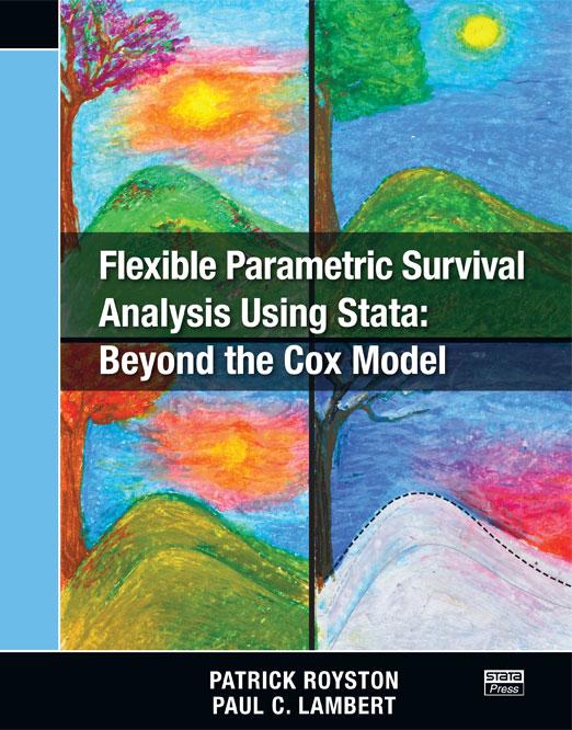
Flexible Parametric Survival Analysis Using Stata: Beyond the Cox Model
106,000원
Authors: Patrick Royston and Paul C. Lambert Publisher: Stata Press Copyright: 2011 ISBN-13: 978-1-59718-079-5 Pages: 347; paperback
Researchers wishing to fit regression models to survival data have long faced the difficult task of choosing between the Cox model and a parametric survival model, such as Weibull. Cox models are fit using Stata’s stcox command, and parametric models are fit using streg, which offers five parametric forms in addition to Weibull. While the Cox model makes minimal assumptions about the form of the baseline hazard function, prediction of hazards and other related functions for a given set of covariates is hindered by this lack of assumptions; the resulting estimated curves are not smooth and do not possess information about what occurs between the observed failure times. Parametric models offer nice, smooth predictions by assuming a functional form of the hazard, but often the assumed form is too structured for use with real data, especially if there exist significant changes in the shape of the hazard over time.
Flexible Parametric Survival Analysis Using Stata: Beyond the Cox Model is concerned with obtaining a compromise between Cox and parametric models that retains the desired features of both types of models. The book is aimed at researchers who are familiar with the basic concepts of survival analysis and with the stcox and streg commands in Stata. As such, it is an excellent complement to An Introduction to Survival Analysis Using Stata by Cleves, Gould, and Marchenko.
This book is written for Stata 12 but is fully compatible with Stata 11 as well.
Much of the text is dedicated to estimation with Royston–Parmar models using the stpm2 command, which is maintained by the authors and available from the Statistical Software Components (SSC) archive at http://www.repec.org. Royston–Parmar models are highly flexible alternatives to the exponential, Weibull, loglogistic, and lognormal models (fit using streg) that allow extension from proportional hazards to proportional odds and to scaled probit models. Additional flexibility is obtained by the use of restricted cubic spline functions as alternatives to the linear functions of log time used in standard models. The authors demonstrate fitting these models and graphing predicted hazards, cumulative hazards, and survival functions with real data from breast cancer and prostate cancer studies.
After some introductory material on the motivation behind flexible parametric models and on working with survival data in Stata, the authors proceed by demonstrating that Cox models may instead be expressed as Poisson models by splitting the time scale at the observed failures. The Poisson-model expression allows for extension by changing how the time scale is split and by introducing restricted cubic splines and fractional polynomials.
Royston–Parmar models are then introduced, followed by material on model building and diagnostics for these models. Considerable attention is then given to time-dependent effects, how these may be modeled, and how to interpret the graphs of the predicted functions that the models produce. This material is followed by a chapter on relative survival models, such as those used for population-based cancer studies. This chapter is very thorough, relates well to the previous material, and is an ideal introduction for those new to the concepts of relative survival and excess mortality. The final chapter is devoted to advanced topics, such as determining the number needed to treat (NNT), handling multiple-event data, and analyzing competing risks.
Patrick Royston is a senior medical statistician at the Medical Research Council, London, UK. He has published research papers on a variety of topics in leading statistics journals. His key interests include multivariable modeling and validation, survival analysis, design and analysis of clinical trials, and statistical computing and algorithms. He is an associate editor of the Stata Journal.
Paul Lambert is a reader in medical statistics at Leicester University, UK. His main interest is in the development and application of statistical methods in population-based cancer research and related fields. He has published widely in leading statistical and medical journals.
1.2 A brief review of the Cox proportional hazards model
1.3 Beyond the Cox model
1.3.2 The baseline hazard contains useful information
1.3.3 Advantages of smooth survival functions
1.3.4 Some requirements of a practical survival analysis
1.3.5 When the proportional-hazards assumption is breached
1.4.2 Time-dependent HRs
1.4.3 Modeling on different scales
1.4.4 Relative survival
1.4.5 Prediction out of sample
1.4.6 Multiple time scales
1.6 A brief introduction to stpm2
1.6.2 Postestimation facilities (prediction)
1.8 Comparing models
1.9 The delta method
1.10 Ado-file resources
1.11 How our book is organized
2.2 Some key concepts
2.3 Syntax of the stset command
2.4 Variables created by the stset command
2.5 Examples of using stset
2.5.2 Using the scale( ) option
2.5.3 Date of diagnosis and date of exit
2.5.4 Date of diagnosis and date of exit with the scale( ) option
2.5.5 Restricting the follow-up time
2.5.6 Left-truncation
2.5.7 Age as the time scale
2.6.2 Time-varying covariates
3.2 Rotterdam breast cancer data
3.3 England and Wales breast cancer data
3.4 Orchiectomy data
3.5 Conclusion
4.2 Modeling rates with the Poisson distribution
4.3 Splitting the time scale
4.3.2 Time as just another covariate
4.5 Splitting at unique failure times
4.7 Fine splitting of the time scale
4.8 Splines: Motivation and definition
4.8.2 Restricted cubic splines
4.8.3 Splines: Application to the Rotterdam data
4.8.4 Varying the number of knots
4.8.5 Varying the location of the knots
4.8.6 Estimating the survival function
4.9.2 Higher order FP models
4.9.3 FP function selection procedure
5.1.2 The Weibull distribution
5.1.3 Generalizing the Weibull
5.1.4 Estimating the hazard function
5.2.2 Example
5.2.3 Comparing parameters of PH(1) and Weibull models
5.4.2 The loglogistic model
5.4.3 Generalizing the loglogistic model
5.4.4 Comparing parameters of PO(1) and loglogistic models
5.5.2 Generalizing the probit model
5.5.3 Comparing parameters of probit(1) and lognormal models
5.5.4 Comments on probit and POs models
5.6.2 Example
5.6.3 Likelihood function and parameter estimation
5.6.4 Comparing regression coefficients
5.6.5 Model selection
5.6.6 Sensitivity to number of knots
5.6.7 Sensitivity to location of knots
6.2 Developing and reporting a prognostic model
6.3 What does the baseline hazard function mean?
6.5.2 Survival probabilities across the risk spectrum
6.5.3 Survival probabilities at given covariate values
6.5.4 Survival probabilities in groups
6.5.5 Plotting adjusted survival curves
6.5.6 Plotting differences between survival curves
6.5.7 Centiles of the survival distribution
6.7.2 Harrell’s C index of concordance
6.8.2 Extrapolation of survival functions: Further investigations
6.8.3 Validation of prognostic models: Basics
6.8.4 Validation of prognostic models: Further comments
7.2 Definitions
7.3 What do we mean by a TD effect?
7.4 Proportional on which scale?
7.5 Poisson models with TD effects
7.5.2 Using restricted cubic splines
7.6.2 Continuous TD effects
7.6.3 More than one TD effect
7.6.4 Stratification is the same as including TD effects
7.8 Attained age as the time scale
7.8.2 Proportional hazards model
7.8.3 TD model
7.10 Prognostic models with TD effects
8.2 What is relative survival?
8.3 Excess mortality and relative survival
8.3.2 Relative survival is a ratio
8.5 Life-table estimation of relative survival
8.6.2 Restricted cubic splines
8.7.2 Proportional cumulative excess hazards
8.7.3 RP models on other scales
8.7.4 Application to England and Wales breast cancer data
8.7.5 Relative survival models on other scales
8.7.6 Time-dependent effects
8.9 Age as a continuous variable
8.10 Concluding remarks
9.2 Number needed to treat
9.4.2 Example 2: CD4 lymphocyte data
9.4.3 Example 3: Prostate cancer data
9.5.2 The AG model
9.5.3 The WLW model
9.5.4 The PWP model
9.5.5 Multiple events in RP models
9.5.6 Summary
9.6.2 The “zeros trick” in WinBUGS
9.6.3 Fitting a RP model
9.6.4 Summary
9.8.2 What is period analysis?
9.8.3 Application to England and Wales breast cancer data
9.9.2 Application to England and Wales breast cancer data
9.9.3 Conclusion

