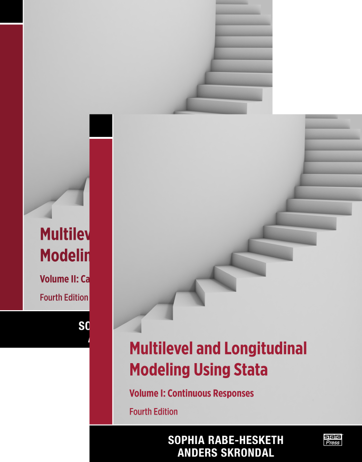
Multilevel and Longitudinal Modeling Using Stata, Fourth Edition
230,000원
Volume I: Continuous Responses
Volume II: Categorical Responses, Counts, and Survival
Authors: Sophia Rabe-Hesketh and Anders Skrondal Publisher: Stata Press Copyright: 2022 ISBN-13: 978-1-59718-108-5 Pages: 974; paperback
Obtain answers to the exercises
Resources for instructors
Read reviews of the first edition
Review of second edition from the Stata Journal
Read reviews of the second editionVolume I: Continuous Responses
ISBN-13: 978-1-59718-137-2 Pages: 554; paperback Author index for Volume I (PDF)
Subject index for Volume I (PDF)
Preface (PDF)
Volume II: Categorical Responses, Counts, and Survival
ISBN-13: 978-1-59718-138-9 Pages: 477; paperback Author index for Volume II (PDF)
Subject index for Volume II (PDF)
Chapter 10—Dichotomous or binary responses (PDF)
Multilevel and Longitudinal Modeling Using Stata, Fourth Edition, by Sophia Rabe-Hesketh and Anders Skrondal, is a complete resource for learning to model data in which observations are grouped—whether those groups are formed by a nesting structure, such as children nested in classrooms, or formed by repeated observations on the same individuals. This text introduces random-effects models, fixed-effects models, mixed-effects models, marginal models, dynamic models, and growth-curve models, all of which account for the grouped nature of these types of data. As Rabe-Hesketh and Skrondal introduce each model, they explain when the model is useful, its assumptions, how to fit and evaluate the model using Stata, and how to interpret the results. With this comprehensive coverage, researchers who need to apply multilevel models will find this book to be the perfect companion. It is also the ideal text for courses in multilevel modeling because it provides examples from a variety of disciplines as well as end-of-chapter exercises that allow students to practice newly learned material.
The book comprises two volumes. Volume I focuses on linear models for continuous outcomes, while volume II focuses on generalized linear models for binary, ordinal, count, and other types of outcomes.
Volume I begins with a review of linear regression and then builds on this review to introduce two-level models, the simplest extensions of linear regression to models for multilevel and longitudinal/panel data. Rabe-Hesketh and Skrondal introduce the random-intercept model without covariates, developing the model from principles and thereby familiarizing the reader with terminology, summarizing and relating the widely used estimating strategies, and providing historical perspective. Once the authors have established the foundation, they smoothly generalize to random-intercept models with covariates and then to a discussion of the various estimators (between, within, and random effects). The authors also discuss models with random coefficients. The text then turns to models specifically designed for longitudinal and panel data—dynamic models, marginal models, and growth-curve models. The last portion of volume I covers models with more than two levels and models with crossed random effects.
The foundation and in-depth coverage of linear-model principles provided in volume I allow for a straightforward transition to generalized linear models for noncontinuous outcomes, which are described in volume II. This second volume begins with chapters introducing multilevel and longitudinal models for binary, ordinal, nominal, and count data. Focus then turns to survival analysis, introducing multilevel models for both discrete-time survival data and continuous-time survival data. The volume concludes by extending the two-level generalized linear models introduced in previous chapters to models with three or more levels and to models with crossed random effects.
In both volumes, readers will find extensive applications of multilevel and longitudinal models. Using many datasets that appeal to a broad audience, Rabe-Hesketh and Skrondal provide worked examples in each chapter. They also show the breadth of Stata's commands for fitting the models discussed. They demonstrate Stata's xt suite of commands (xtreg, xtlogit, xtpoisson, etc.), which is designed for two-level random-intercept models for longitudinal/panel data. They demonstrate the me suite of commands (mixed, melogit, mepoisson, etc.), which is designed for multilevel models, including those with random coefficients and those with three or more levels. In volume 2, they discuss gllamm, a community-contributed Stata command developed by Rabe-Hesketh and Skrondal that can fit many latent-variable models, of which the generalized linear mixed-effects model is a special case.The types of models fit by the xt commands, the me commands, and gllamm sometimes overlap; when this happens, the authors highlight the differences in syntax, data organization, and output for the commands. The authors also point out the strengths and weaknesses of these commands, based on considerations such as computational speed, accuracy, available predictions, and available postestimation statistics.
The fourth edition of Multilevel and Longitudinal Modeling Using Stata has been thoroughly revised and updated. In it, you will find new material on Kenward–Roger degrees-of-freedom adjustments for small sample sizes, difference-in-differences estimation for natural experiments, instrumental-variables estimation to account for level-one endogeneity, and Bayesian estimation for crossed-effects models. In addition, you will find new discussions of meologit, cmxtmixlogit, mestreg, menbreg, and other commands introduced in Stata since the third edition of the book.
In summary, Multilevel and Longitudinal Modeling Using Stata, Fourth Edition is the most complete, up-to-date depiction of Stata’s capacity for fitting models to multilevel and longitudinal data. Readers will also find thorough explanations of the methods and practical advice for using these techniques. This text is a great introduction for researchers and students wanting to learn about these powerful data analysis tools.
Sophia Rabe-Hesketh is a professor of educational statistics and biostatistics at the University of California at Berkeley and a chair of social statistics at the Institute of Education, University of London.
Anders Skrondal is a senior biostatistician at the Division of Epidemiology, Norwegian Institute of Public Health. He was previously a professor of statistics and director of the Methodology Institute at the London School of Economics and a professor of biostatistics at the University of Oslo.
1.2 Is there gender discrimination in faculty salaries?
1.3 Independent-samples t test
1.4 One-way analysis of variance
1.5 Simple linear regression
1.6 Dummy variables
1.7 Multiple linear regression
1.8 Interactions
1.9 Dummy variables for more than two groups
1.10 Other types of interactions
1.10.2 Interaction between continuous covariates
1.12 Residual diagnostics
1.13 Causal and noncausal interpretations of regression coefficients
1.13.2 Regression as structural model
1.15 Exercises
2.2 How reliable are peak-expiratory-flow measurements?
2.3 Inspecting within-subject dependence
2.4 The variance-components model
2.4.2 Path diagram
2.4.3 Between-subject heterogeneity
2.4.4 Within-subject dependence
Intraclass correlation versus Pearson correlation
2.5.2 Using xtreg
2.5.3 Using mixed
2.6.2 Hypothesis test and confidence interval for the between-cluster variance
Score test
F test
Confidence interval
2.8 Fixed versus random effects
2.9 Crossed versus nested effects
2.10 Parameter estimation
Distributional assumptions
2.10.3 Inference for β
Estimate: Unbalanced case
Implementation via the mean total residual
2.11.3 Empirical Bayes standard errors
Diagnostic standard errors
Accounting for uncertainty in β̂
2.11.4 Bayesian interpretation of REML estimation and prediction
2.13 Exercises
3.2 Does smoking during pregnancy affect birthweight?
3.3.2 Model assumptions
3.3.3 Mean structure
3.3.4 Residual covariance structure
3.3.5 Graphical illustration of random-intercept model
3.4.2 Using mixed
3.6 Hypothesis tests and confidence intervals
3.6.2 Joint hypothesis tests for several regression coefficients
3.6.3 Predicted means and confidence intervals
3.6.4 Hypothesis test for random-intercept variance
3.7.2 Within-mother effects
3.7.3 Relations among estimators
3.7.4 Level-2 endogeneity and cluster-level confounding
3.7.5 Allowing for different within and between effects
3.7.6 Robust Hausman test
3.9 Assigning values to random effects: Residual diagnostics
3.10 More on statistical inference
Feasible generalized least squares (FGLS)
ML by iterative GLS (IGLS)
ML by Newton-Raphson and Fisher scoring
ML by the expectation-maximization (EM) algorithm
REML
Purely within-cluster covariate
Purely within-cluster covariate
3.12 Exercises
4.2 How effective are different schools?
4.3 Separate linear regressions for each school
4.4 Specification and interpretation of a random-coefficient model
4.4.2 Interpretation of the random-effects variances and covariances
4.5.2 Random-coefficient model
4.7 Interpretation of estimates
4.8 Assigning values to the random intercepts and slopes
4.8.2 Empirical Bayes prediction
4.8.3 Model visualization
4.8.4 Residual diagnostics
4.8.5 Inferences for individual schools
4.10 Some warnings about random-coefficient models
4.10.2 Many random coefficients
4.10.3 Convergence problems
4.10.4 Lack of identification
4.12 Exercises
5.2 Random-effects approach: No endogeneity
5.3 Fixed-effects approach: Level-2 endogeneity
Subject dummies
5.3.3 Mundlak approach and robust Hausman test
5.3.4 First-differencing
5.4.2 Repeated-measures ANOVA
5.5.2 Fixed-coefficient model: Level-2 endogeneity
5.7 Instrumental-variable methods: Level-1 (and level-2) endogeneity
5.7.2 Conventional fixed-effects approach
5.7.3 Fixed-effects IV estimator
5.7.4 Random-effects IV estimator
5.7.5 More Hausman tests
5.8.2 Dynamic model with subject-specific intercepts
5.10 Exercises
6.2 Mean structure
6.3 Covariance structures
6.3.2 Random-intercept or compound symmetric/exchangeable structure
6.3.3 Random-coefficient structure
6.3.4 Autoregressive and exponential structures
6.3.5 Moving-average residual structure
6.3.6 Banded and Toeplitz structures
6.4.2 Heteroskedastic level-1 residuals over occasions
6.4.3 Heteroskedastic level-1 residuals over groups
6.4.4 Different covariance matrices over groups
6.6 Generalized estimating equations (GEE)
6.7 Marginal modeling with few units and many occasions
6.7.2 Marginal modeling for long panels
6.7.3 Fitting marginal models for long panels in Stata
6.9 Exercises
7.2 How do children grow?
Predicting the mean trajectory
Predicting trajectories for individual children
Predicting the mean trajectory
7.5 Heteroskedasticity
7.5.2 Heteroskedasticity at level 2
7.7 Growth-curve model as a structural equation model
7.7.2 Estimation using mixed
7.9 Exercises
8.2 Do peak-expiratory-flow measurements vary between methods within subjects?
8.3 Inspecting sources of variability
8.4 Three-level variance-components models
8.5 Different types of intraclass correlation
8.6 Estimation using mixed
8.7 Empirical Bayes prediction
8.8 Testing variance components
8.9 Crossed versus nested random effects revisited
8.10 Does nutrition affect cognitive development of Kenyan children?
8.11 Describing and plotting three-level data
8.11.2 Level-1 variables
8.11.3 Level-2 variables
8.11.4 Level-3 variables
8.11.5 Plotting growth trajectories
8.12.2 Model specification: Three-stage formulation
8.12.3 Estimation using mixed
8.15 Summary and further reading
8.16 Exercises
9.2 How does investment depend on expected profit and capital stock?
9.3 A two-way error-components model
9.3.2 Residual variances, covariances, and intraclass correlations
Cross-sectional correlations
9.3.4 Prediction
9.5 Data structure
9.6 Additive crossed random-effects model
9.6.2 Intraclass correlations
9.6.3 Estimation using mixed
9.7.2 Intraclass correlations
9.7.3 Estimation using mixed
9.7.4 Testing variance components
9.7.5 Some diagnostics
9.9 Summary and further reading
9.10 Exercises
10.2 Single-level logit and probit regression models for dichotomous responses
Estimation using logit
Estimation using glm
Probit regression
Estimation using probit
10.4 Longitudinal data structure
10.5 Proportions and fitted population-averaged or marginal probabilities
Two-stage formulation
10.6.3 Estimation
Using melogit
Using gllamm
10.8 Measures of dependence and heterogeneity
10.8.2 Median odds ratio
10.8.3 Measures of association for observed responses at median fixed part of the model
10.9.2 Tests of variance components
10.10.2 Some speed and accuracy considerations
Starting values
Using melogit and gllamm for collapsible data
Spherical quadrature in gllamm
10.11.2 Empirical Bayes prediction
10.11.3 Empirical Bayes modal prediction
10.12.2 Predicted subject-specific probabilities
Predictions for the subjects in the sample: Posterior mean probabilities
10.15 Exercises
11.2 Single-level cumulative models for ordinal responses
11.2.2 Latent-response formulation
11.2.3 Proportional odds
11.2.4 Identification
11.4 Longitudinal data structure and graphs
11.4.2 Plotting cumulative proportions
11.4.3 Plotting cumulative sample logits and transforming the time scale
Estimation using gllamm
Median odds ratio
Estimation using gllamm
11.8.2 Predicted subject-specific probabilities: Posterior mean
11.10 A random-intercept probit model with grader bias
Continuation-ratio logit model
Adjacent-category logit model
Baseline-category logit and stereotype models
11.15 Exercises
12.2 Single-level models for nominal responses
Estimation using mlogit
Estimation using clogit
Estimation using cmclogit
Estimation using cmclogit
12.4 Utility-maximization formulation
12.5 Does marketing affect choice of yogurt?
12.6 Single-level conditional logit models
Estimation using cmclogit
Estimation using gllamm
Estimation using gllamm
Estimation using gllamm
12.9 Prediction of random effects and household-specific choice probabilites
12.10 Summary and further reading
12.11 Exercises
13.2 What are counts?
13.2.2 Counts as aggregated event-history data
13.4 Did the German healthcare reform reduce the number of doctor visits?
13.5 Longitudinal data structure
13.6 Single-level Poisson regression
Estimation using glm
13.7.2 Measures of dependence and heterogeneity
13.7.3 Estimation
Using mepoisson
Using gllamm
Estimation using gllamm
Constant dispersion or NB1
13.10.3 Negative binomial models with random intercepts
Estimation using Poisson regression with dummy variables for clusters
13.11.3 Generalized estimating equations
13.14 Standardized mortality ratios
13.15 Random-intercept Poisson regression
13.18 Exercises
14.2 Single-level models for discrete-time survival data
14.2.3 Estimation via regression models for dichotomous responses
14.4 Data expansion
14.5 Proportional hazards and interval-censoring
14.6 Complementary log&endash;log models
14.9 Summary and further reading
14.10 Exercises
15.2 What makes marriages fail?
15.3 Hazards and survival
15.4 Proportional hazards models
Estimation using poisson
Estimation using stintreg
15.8 Marginal modeling
15.12.2 Counting process risk interval
15.12.3 Gap-time risk interval
15.14 Exercises
16.2 Did the Guatemalan-immunization campaign work?
16.3 A three-level random-intercept logistic regression model
16.3.2 Measures of dependence and heterogeneity
Types of median odds ratios
16.3.4 Estimation
Using gllamm
Using gllamm
16.5.2 Empirical Bayes modal prediction
16.6.2 Predicted median or conditional probabilities
16.6.3 Predicted posterior mean probabilities: Existing clusters
16.8 Crossed random-effects logistic regression
16.8.2 Approximate maximum likelihood estimation
Priors for the salamander data
Estimation using bayes: melogit
16.8.5 Fully Bayesian versus empirical Bayesian inference for random effects
16.10 Exercises

